The existence of antimatter became known following Dirac’s formulation of relativistic quantum mechanics, but this incredible development was not anticipated. These days conjuring up a new particle or field (or perhaps even new dimensions) to explain unknown observations is pretty much standard operating procedure, but it was not always so. The famous “who ordered that” statement of I. I. Rabi was made in reference to the discovery of the muon, a heavy electron whose existence seemed a bit unnecessary at the time; in fact it was the harbinger of a subatomic zoo.
The story of Dirac’s relativistic reformulation of the Schrödinger wave equation, and the subsequent prediction of antiparticles, is particularly appealing; the story is nicely explained in a recent biography of Dirac (Farmelo 2009). As with Einstein’s theory of relativity, Dirac’s relativistic quantum mechanics seemed to spring into existence without any experimental imperative. That is to say, nobody ordered it! The reality, of course, is a good deal more complicated and nuanced, but it would not be inaccurate to suggest that Dirac was driven more by mathematical aesthetics than experimental anomalies when he developed his theory.
The motivation for any modification of the Schrödinger equation is that it does not describe the energy of a free particle in a way that is consistent with the special theory of relativity. At first sight it might seem like a trivial matter to simply re-write the equation to include the energy in the necessary form, but things are not so simple. In order to illustrate why this is so it is instructive to briefly consider the Dirac equation, and how it was developed. For explicit mathematical details of the formulation and solution of the Dirac equation see, for example, Griffiths 2008.
The basic form of the Schrödinger wave equation (SWE) is
 (1)
(1)
The fundamental departure from classical physics embodied in eq (1) is the quantity  , which represents not a particle but a wavefunction. That is, the SWE describes how this wavefunction (whatever it may be) will behave. This is not the same thing at all as describing, for example, the trajectory of a particle. Exactly what a wavefunction is remains to this day rather mysterious. For many years it was thought that the wavefunction was simply a handy mathematical tool that could be used to describe atoms and molecules even in the absence of a fully complete theory (e.g., Bohm 1952). This idea, originally suggested by de Broglie in his “pilot wave” description, has been disproved by numerous ingenious experiments (e.g., Aspect et al., 1982). It now seems unavoidable to conclude that wavefunctions represent actual descriptions of reality, and that the “weirdness” of the quantum world is in fact an intrinsic part of that reality, with the concept of “particle” being only an approximation to that reality, only appropriate to a coarse-grained view of the world. Nevertheless, by following the rules that have been developed regarding the application of the SWE, and quantum physics in general, it is possible to describe experimental observations with great accuracy. This is the primary reason why many physicists have, for over 80 years, eschewed the philosophical difficulties associated with wavefunctions and the like, and embraced the sheer predictive power of the theory.
We will not discuss quantum mechanics in any detail here; there are many excellent books on the subject at all levels (e.g., Dirac 1934, Shankar 1994, Schiff 1968). In classical terms the total energy of a particle E can be described simply as the sum of the kinetic energy (KE) and the potential energy (PE) as
 (2)
(2)
where p = mv represents the momentum of a particle of mass m and velocity v. In quantum theory such quantities are described not by simple formulae, but rather by operators that act on the wavefunction. We describe momentum via the operator  and energy by
  and so on. The first term of eq (1) represents the total energy of the system, and is also known as the Hamiltonian, H. Thus, the SWE may be written as
 (3)
(3)
The reason why eq (3) is non-relativistic is that the energy-momentum relation in the Hamiltonian is described in the well-known non-relativistic form. As we know from Einstein, however, the total energy of a free particle does not reside only in its kinetic energy; there is also the rest mass energy, embodied in what may be the most famous equation in all of physics:
 (4)
(4)
This equation tells us that a particle of mass m has an equivalent energy E, with c2 being a rather large number, illustrating that even a small amount of mass (m) can, in principle, be converted into a very large amount of energy (E). Despite being so famous as to qualify as a cultural icon, the equation E = mc2 is, at best, incomplete. In fact the total energy of a free particle (i.e., V = 0) as prescribed by the theory of relativity is given by
 (5)
(5)
Clearly this will reduce to E = mc2 for a particle at rest (i.e., p = 0): or will it? Actually, we shall have E = ± mc2, and in some sense one might say that the negative solutions to this energy equation represent antimatter, although, as we shall see, the situation is not so clear cut. In order to make the SWE relativistic then, one need only replace the classical kinetic energy E = p2/2m with the relativistic energy E = [m2c4+p2c2]1/2. This sounds simple enough, but the square root sign leads to quite a lot of trouble! This is largely because when we make the “quantum substitution”  we find we have to deal with the square root of an operator, which, as it turns out, requires some mathematical sophistication. Moreover, in quantum physics we must deal with operators that act upon complex wavefunctions, so that negative square roots may in fact correspond to a physically meaningful aspect of the system, and cannot simply be discarded as might be the case in a classical system.
To avoid these problems we can instead start with eq (5) interpreted via the operators for momentum and energy so that eq (3) becomes
 (6)
(6)
This equation is known as the Klein Gordon equation (KGE), although it was first obtained by Schrödinger in his original development of the SWE. He abandoned it, however, when he found that it did not properly describe the energy levels of the hydrogen atom. It subsequently became clear that when applied to electrons this equation also implied two things that were considered to be unacceptable; negative energy solutions, and, even worse, negative probabilities. We now know that the KGE is not appropriate for electrons, but does describe some massive particles with spin zero when interpreted in the framework of quantum field theory (QFT); neither mesons nor QFT were known when the KGE was formulated.
Some of the problems with the KGE arise from the second order time derivative, which is itself a direct result of squaring everything to avoid the intractable mathematical form of the square root of an operator. The fundamental connection between time and space at the heart of relativity leads to a similar connection between energy and momentum, a connection that is overlooked in the KGE. Dirac was thus motivated by the principles of relativity to keep a first order time derivative, which meant that he had to confront the difficulties associated with using the relativistic energy head on. We will not discuss the details of its derivation but will simply consider the form of the resulting Dirac equation:
 (7)
(7)
This equation has the general form of the SWE, but with some significant differences. Perhaps the most important of these is that the Hamiltonian now includes both the kinetic energy and the electron rest mass, but the coefficients αi and  have to be four-component matrices to satisfy the equation. That is, the Dirac equation is really a matrix equation, and the wavefunction it describes must be a four component wavefunction. Although there are no problems with negative probabilities, the negative energy solutions seen in the KGE remain. These initially seemed to be a fatal flaw in Dirac’s work, but were overlooked because in every other aspect the equation was spectacularly successful. It reproduced the hydrogen atomic spectra perfectly (at least, as perfectly as it was known at the time) and even included small relativistic effects, as a proper relativistic wave equation should. For example, when the electromagnetic interaction is included the Dirac equation predicts an electron magnetic moment:
 (8)
(8)
where  is known as the Bohr magneton. This expression is also in agreement with experiment, almost: it was later discovered that the magnetic moment of the electron differs from the value predicted by eq (8) by about 0.1% (Kusch and Foley 1948). The fact that Dirac’s theory was able to predict these quantities was considered to be a triumph, despite the troublesome negative energy solutions.
Another intriguing aspect of the Dirac equation was noticed by Schrödinger in 1930. He realised that interference between positive and negative energy terms would lead to oscillations of the wavepacket of an electron (or positron) about some central point at the speed of light. This fast motion was given the name zitterbewegung (which is German for “trembling motion”). The underlying physical mechanism that gives rise to the zitterbewegung effect may be interpreted in several different ways but one way to look at it is as an interaction of the electron with the zero-point energy of the (quantised) electromagnetic field. Such electronic oscillations have not been directly observed as they occur at a very high frequency (~ 1021 Hz), but since zitterbewegung also applies to electrons bound to atoms, this motion can affect atomic energy levels in an observable way. In a hydrogen atom the zitterbewegung acts to “smear out” the electron charge over a larger area, lowering the strength of its interaction with the proton charge. Since S states have a non-zero expectation value at the origin, the effect is larger for these than it is for P states. The splitting between the hydrogen 2S1/2 and 2P1/2 states, that are degenerate in the Dirac theory, is known as the Lamb Shift (Lamb, 1947). This shift, which amounts to ~1 GHz was observed in an experiment by Willis Lamb and his student Robert Retherford (not to be confused Ernest Rutherford!). The need to explain this shift, which requires a proper explanation of the electron interacting with the electromagnetic field, gave birth to the theory of quantum electrodynamics, pioneered by Bethe, Tomanoga, Schwinger and Feynman.
The solutions to the SWE for free particles (i.e., neglecting the potential V) are of the form
 (9)
(9)
Here A is some function that depends only on the spatial properties of the wavefunction (i.e., not on t). Note that this wavefunction represents two electron states, corresponding to the two separate spin states. The corresponding solutions to the Dirac equation may be represented as
 (10)
(10)
Here  represents the negative energy solutions that have caused so much trouble. The existence of these states is central to the theory they cannot simply be labelled as “unphysical” and discarded. The complete set of solutions is required in quantum mechanics, in which everything is somewhat “unphysical”. More properly, since the wavefunction is essentially a complex probability density function that yields a real result when its absolute value is squared, the negative energy solutions are no less physical than the positive energy solutions; it is in fact simply a matter of convention as to which states are positive and which are negative. However you set things up, you will always have some “wrong” energy states that you can’t get rid of. Thus, Dirac was able to eliminate the negative probabilities and produce a wave equation that was consistent with special relativity, but the negative energy states turned out to be a fundamental part of the theory and could not be eliminated, despite many attempts to get rid of them.
After his first paper in 1928 (The quantum theory of the electron) Dirac had established that his equation was a viable relativistic wave equation, but the negative energy aspects remained controversial. He worried about this for some time, and tried to develop a “hole” theory to explain their seemingly undeniable existence. A serious problem with negative energy solutions is that one would expect all electrons to decay into the lowest energy state available, which would be the negative energy states. Since this would not be consistent with observations there must, so Dirac reasoned, be some mechanism to prevent it. He suggested that the states were already filled with an infinite “sea” of electrons, and therefore the Pauli Exclusion Principle would prevent such decay, just as it prevents more than two electrons from occupying the lowest energy level in an atom. (Note that this scheme does not work for Bosons, which do not obey the exclusion principle). Such an infinite electron sea would have no observable properties, as long as the underlying vacuum has a positive “bare” charge to cancel out the negative electron charge. Since only changes in the energy density of this sea would be apparent, we would not normally notice its presence. Moreover, Dirac suggested that if a particle were missing from the sea the resulting hole would be indistinguishable from a positively charged particle, which he speculated was a proton, protons being the only positively charged subatomic particles known at the time.
This idea was presented in a paper in 1930 (A Theory of Electrons and Protons, Dirac 1930). The theory was less than successful, however, and the deficiencies served only to undermine confidence in the entire Dirac theory. Attempts to identify holes as protons only made matters worse; it was shown independently by Heisenberg, Oppenheimer and Pauli that the holes must have the electron mass, but of course protons are almost 2000 times heavier. Moreover, the instability between electrons and holes completely ruled out stable atomic states made from these entities (bad news for hydrogen, and all other atoms). Eventually Dirac was forced to conclude that the negative energy solutions must correspond to real particles with the same mass as the electron and a positive charge. He called these anti-electrons (Quantised Singularities in the Electromagnetic Field, Dirac 1931).
This almost reluctant conclusion was not based on a full understanding of what the negative energy states were, but rather the fact that the entire theory, which was so beautiful in other ways that it was hard to resist, depended on them. It turns out that to properly understand the negative energy solutions requires the formalism of quantum field theory (QFT). In this description particles (and antiparticles) can be created or destroyed, so it is no longer necessarily appropriate to consider these particles to be the fundamental elements of the theory. If the total number of particles in a system is not conserved then one might prefer to describe that system in terms of the entities that give rise to the particles rather than the particles themselves. These are the quantum fields, and the standard model of particle physics is at its heart a QFT. By describing particles as oscillations in a quantum field not only do we have an immediate mechanism by which they may be created or destroyed, but the problem of negative energies is also removed, as this simply becomes a different kind of variation in the underlying quantum field. Dirac didn’t explicitly know this at the time, although it would be fair to say that he essentially invented QFT, when he produced a quantum theory that included quantized electromagnetic fields (Dirac, 1927, The Quantum Theory of the Emission and Absorption of Radiation). This led, eventually, to what would be known as quantum electrodynamics. Dirac would undoubtedly have been able to make much more use of his creation if he had not been so appalled by the notion of renormalization. Unfortunately this procedure, which in some ways can be thought of as subtracting infinite quantities from each other to leave a finite quantity, was incompatible with his sense of mathematical aesthetics.
So, despite initially struggling with the interpretation of his theory, there can be no question that Dirac did indeed explicitly predict the existence of the positron before it was experimentally observed. This observation came almost immediately in cloud chamber experiments conducted by Carl Anderson in California (C. D. Anderson: The apparent existence of easily deflectable positives, Science 76 238, 1932). Curiously, however, Anderson was not aware of the prediction, and the proximity of the observation was apparently coincidental. We will discuss this remarkable observation in a later post.
*This post is adapted from an as-yet unpublished book chapter by D. B. Cassidy and A. P. Mills, Jr.
References:
Griffiths, D. (2008). Introduction to Elementary Particles Wiley-VCH; 2nd edition.
Farmelo, “The Strangest Man: The Hidden Life of Paul Dirac, Mystic of the Atom” Basic Books, New York, (2011).
Dirac, P.A.M. (1927). The Quantum Theory of the Emission and Absorption of Radiation, Proceedings of the Royal Society of London, Series A, Vol. 114, p. 243.
P. A. M. Dirac, Proc. Phys. Soc. London Sect. A 117, 610 (1928).
P. A. M. Dirac, Proc. Phys. Soc. London Sect. A 126, 360 (1930).
P. A. M. Dirac, Proc. Phys. Soc. London Sect. A 133, 60 (1931).
Anderson, C. D. (1932). The apparent existence of easily deflectable positives, Science 76, 238.
A. Aspect, D. Jean, R. Gerard (1982). Experimental Test of Bell’s Inequalities Using Time- Varying Analyzers, Phys. Rev. Lett. 49 1804
P. Kusch and H. M. Foley “The Magnetic Moment of the Electron”, Phys. Rev. 74, 250 (1948).


 excitation scheme
  Ps atoms are long-lived and could potentially be used for (anti)-gravity measurements, however, the intermediate state (
 ) has interesting properties of it’s own, as described in our latest article
  ) of the electron and positron can combine in positronium to either cancel (
 ) or sum (
 ), depending on the relative alignment between the two components. In the former case (para-Ps) the atom has a very short ground-state lifetime of just 125 ps, whereas in the latter case (ortho-Ps) the atom lives in the
  state for an average of 142 ns (this may not sound very long but it’s actually plenty of time to do spectroscopy with pulsed lasers).
 ) atoms then excite these using 243 nm laser light from our
  and
and  ) dictate that this single-photon transition drives the atoms to the
  ,
,  ,
,  state (
 ). For historical reasons the
  (
( ) and
) and  (
( states have a fluorescence lifetime of 3.19 ns, and an annihilation lifetime of over 100
  s (practically infinite compared to the time-scale of our measurements, i.e.,
  states don’t annihilate directly, but can decay to a different state then annihilate). The
  ortho and para states have annihilation lifetimes of 1136 ns and 1 ns, and they both fluoresce with a lifetime of
  0.24 s (
 ). The bottom line here is that there are a wide range of fluorescence and annihilation lifetimes for the various possible sub-states in the
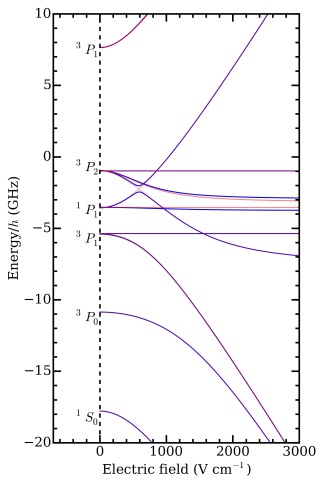
  ) are mixed together (Zeeeman mixing). Similarly, an electric field mixes states with different
  states are subsequently populated. More specifically, if the laser polarization is parallel to the applied magnetic field then only
  transitions are allowed, whereas if the polarization is perpendicular to it then
  must change by
  .
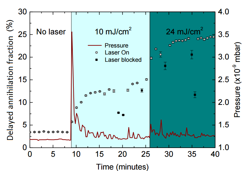
. So what can we actually measure? In most cases, laser excitation makes it more likely for ground state ortho-Ps to ultimately end up in the short-lived para-Ps state, thus applying the laser causes an increase in the annihilation gamma ray flux at early times. This change can be observed and quantified using the parameter
 state. This could be used to produce an ensemble of pure

