Ps spectroscopy

Microwaves & Positronium Pt. III: Positronium Spectroscopy Cubed

Published on April 3, 2024April 3, 2024 by R E SheldonLeave a comment

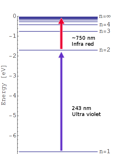
A series of previous posts (found here, here and over here) described how our measurements of the positronium (Ps, an atom formed of an electron and its antimatter counterpart, the positron) 2 ³S₁ → 2 ³P_J fine structure energy intervals were subject to significant shifts due to frequency dependent microwave power [1,2]. This variation in the power was due to reflections of the microwave radiation causing more power at some frequencies that others, skewing our measurements [3,4]. See the previous posts for a description of how we measure line shapes to determine the transition frequency. This post describes a new measurement of the 2 ³S₁ → 2 ³P₂ energy interval, known as the ν₂ transition, performed using a waveguide with a new experimental design to eliminate reflection effects. The full published version of this work can be found in Reference [5].

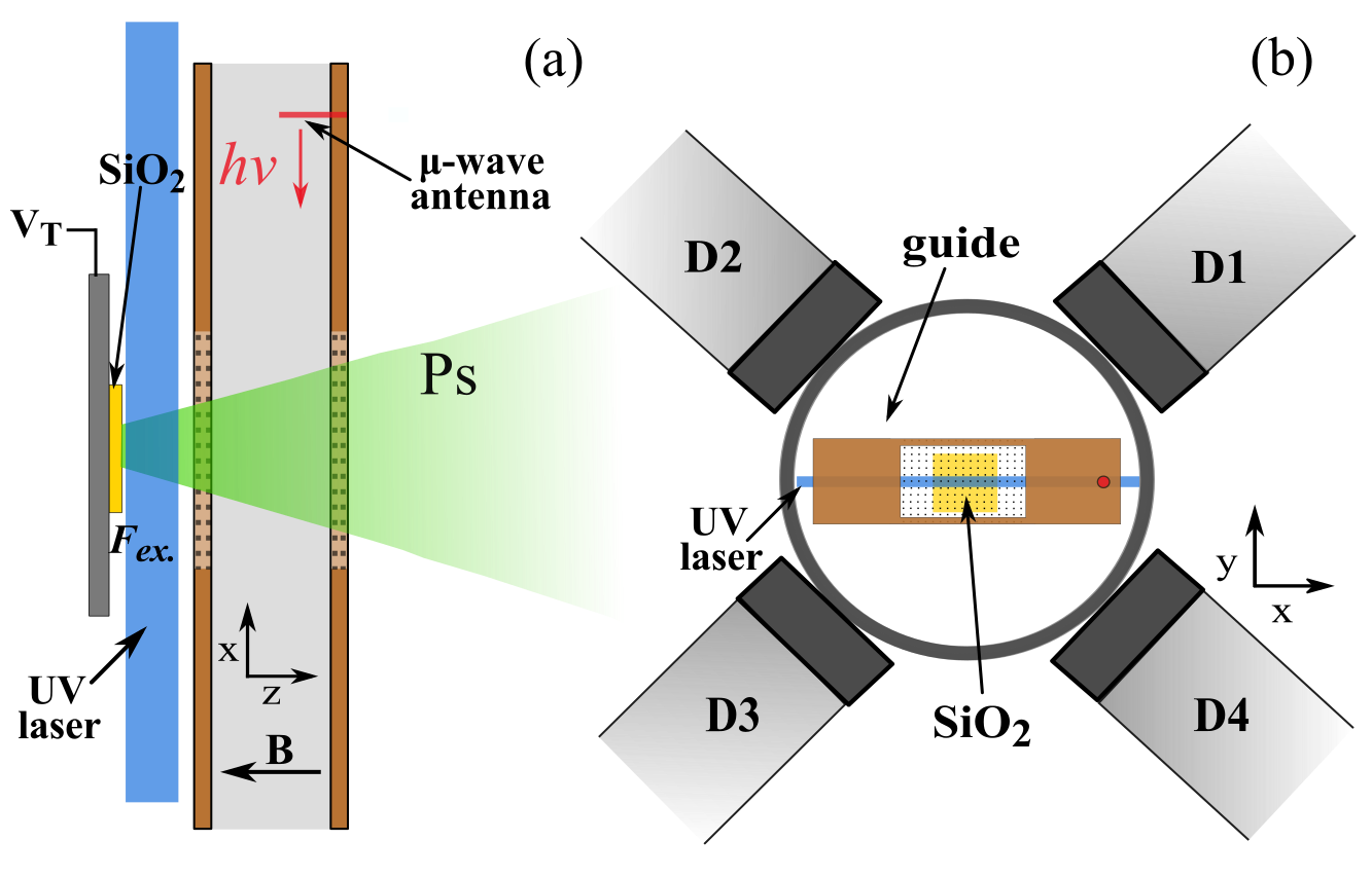
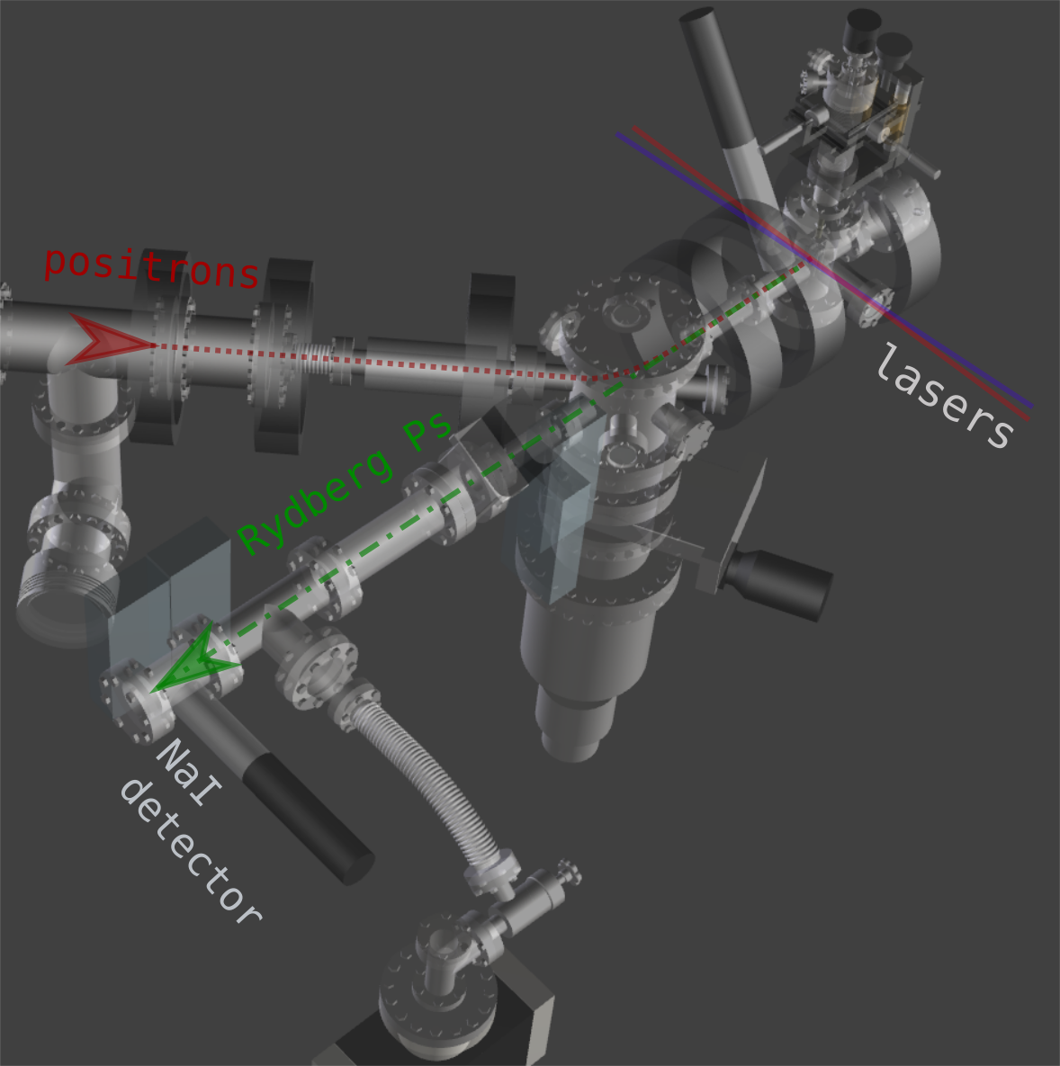
The solution to the reflection problem, as determined from simulations of the microwave fields, was to use a vacuum chamber that minimised the possibility of microwave reflections going back into the waveguide and creating frequency dependent power variation (all our experiments are performed in a vacuum at <0.00000001% of atmospheric pressure to prevent the Ps scattering and annihilating). The vacuum chamber chosen was a cube, see Figure 1 for a diagram of the experimental layout. In this chamber the ends of the waveguide are just a few millimeters from the windows used to let in laser radiation, thus microwaves will pass out of the chamber as fused silica is transparent to microwaves, unlike metal which is highly reflective. This way we reduced the amount of reflected radiation and thus the frequency dependent power variation. Microwave absorbing foam with a reflectivity of <1% was placed on the windows, ensuring no microwaves were reflected back into the waveguide from outside the vacuum chamber.

**Figure 1** A schematic diagram of the experimental setup showing the Ps (green) passing through the waveguide with the microwave absorbing foam (blue) at its exits. Adapted from Reference [5].

This experiment also had a few other improvements. Firstly, Doppler effects were minimised by retro-reflection of the UV laser beam used to make the 2 ³S₁ state Ps. If the laser Doppler selects atoms moving in one direction (away or towards the laser), then the retro-reflected beam, moving in an equal and opposite path, will select out atoms moving in the equal and opposite direction, resulting in a net zero velocity. Secondly, an extra wire mesh E_G was included between the Ps production target E_T, which has a large bias of -3.5 kV, and the waveguide to minimise electric field penetration into the microwave excitation region. Electric fields induce unwanted Stark shifts to ν₂, but are attenuated strongly by wire meshes [6].

The quantum electrodynamic (QED) calculations we wish to test are for the zero-field case, where the atoms are in a region of no electric or magnetic field and do not interact with each other. The atoms in our experiment were a gas with less than 10⁵ atoms per cubed centimeter and the electric fields present were very small. However, our experiment had to take place in a substantial magnetic field because this is how we guide our pulses of positrons to the location where we make Ps. A magnetic field will change the energy of quantum states (i.e. shifting where they lie in the electric potential well of the atom) and thus the energy intervals between states. This is called the Zeeman shift, and it is caused by an applied magnetic field distorting and polarising the probability distribution of the particles [7].

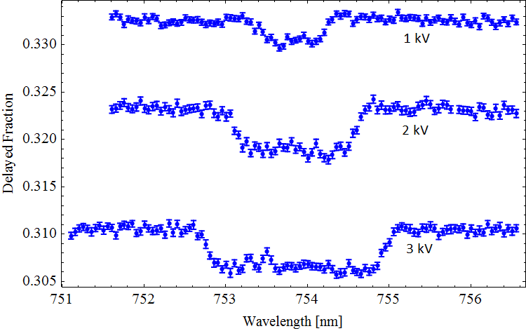
To get around this we measured the transition energy in multiple magnetic fields. The Zeeman shift is quadratic and could be extrapolated back to zero-field to obtain a value to compare with QED calculations. The measured transition energy ν_R (in MHz) is shown in Figure 2 as a function of magnetic field and the dashed lines are the extrapolations to zero-field. The figure shows data for microwave radiation moving toward the Ps atoms in two opposite directions, +x and –x, propagating in either direction along the waveguide. By taking the average of these two measurements we exactly cancel out any Doppler shifts between Ps and microwaves. However, the maximum Doppler shifts was expected to be ±0.26 MHz, based on the maximum possible misalignment of the Ps, laser and waveguide. This is much smaller than the 1.8 MHz difference observed, which is puzzling.

**Figure 2** The measured Zeeman shifted transition frequency extrapolated back to zero field. The blue squares are the transition measured with microwave radiation travelling in the positive x direction, while the red circles are for the negative x direction. The green line and shaded band indicates the average measured zero-field transition frequency and its uncertainty. Hollow points are with microwave foam present and solid points are without microwave foam present. Adapted from Reference [5].

All other systematic effects are <0.1 MHz, yet the two directions disagree with each other. The prime suspect for this shift, reflection effects, was eliminated with the new chamber design and the foam. This was confirmed as shown in Figure 2 whereby data with foam (hollow points) and without foam (solid points) present does not display any change in the measured transition frequency. However, there was a small asymmetry to our line shape mesurements, which has previously indicated frequency dependent power [2]. This lead us to conclude that there were internal effects from defects in the waveguide construction or microwave circuit which caused frequency dependent power, distorting the line shapes. We treated this effect as a systematic error with a magnitude of 1.8/2 = 0.9 MHz, lowering the precision of our final result.

Our final value for the ν₂ energy interval was 8627.94 ± 0.95 MHz, close enough to theory to be in broad agreement, as shown in Figure 3. This new value is the most precise measurement to date but fails to test the latest set of QED calculations, which can be described by a summation of smaller and smaller terms (i.e. ν₂ = O₄ + O₅ + O₆ + O₇ + …). A measurement with just a ten times improvement in precision will be able to do this, and a 10000 times improvement would allow us to to test certain dark matter candidates [2]. We believe that this method has inherent vulnerabilities to frequency dependent microwave power and that other methods should be explored, a post on this will be coming soon. However, with improvements to the waveguide design and microwave circuit this methodology can be used for precision measurements nonetheless.

**Figure 3** A comparison of our measurement of ν₂ with historical ones, including the average of all the measurements so far. The vertical black line and shaded bar is the latest QED calculation and its associated error. Adapted from Reference [5].

[1] Precision Microwave Spectroscopy of the Positronium n = 2 Fine Structure. L. Gurung, T. J. Babij, S. D. Hogan and D. B. Cassidy; Phys. Rev. Lett.125, 073002 (2020)

[2] Observation of asymmetric line shapes in precision microwave spectroscopy of the positronium 2³P₁ →2³P_J (J = 1, 2) fine-structure intervals. L. Gurung, T. J. Babij, J. Pérez-Ríos, S. D. Hogan and D. B. Cassidy; Phys. Rev. A.103, 042805 (2021)

[3] Line-shape modelling in microwave spectroscopy of the positronium n = 2 fine-structure intervals. L. A. Akopyan, T. J. Babij, K. Lakhmanskiy, D. B. Cassidy and A. Matveev; Phys. Rev. A. 104, 062810 (2021)

[4] Microwave spectroscopy of positronium atoms in free space. R. E. Sheldon, T. J. Babij, S. H. Reeder, S. D. Hogan, and D. B. Cassidy; Phys. Rev. A 107, 042810 (2023)

[5] Precision microwave spectroscopy of the positronium 2 ³S₁ →2 ³P₂ interval. R. E. Sheldon, T. J. Babij, S. H. Reeder, S. D. Hogan, and D. B. Cassidy; Phys. Rev. Lett. 131, 043001 (2023)

[6] Penetration of electrostatic fields and potentials through meshes, grids, or gauzes. F. H. Read, N. J. Bowring, P. D. Bullivant, and R. R. A. Ward; Rev. Sci. Instruments, 69 (5), 2000–2006 (1998)

[7] Atomic physics. C. J. Foot; Oxford master series in physics, Oxford University Press (2005)

Microwaves & Positronium Pt. II: Giving Positronium the Horn (Antenna)

Published on March 6, 2024April 24, 2024 by R E Sheldon1 Comment

A previous post of ours (found here) described how our measurements of the energy intervals of the n = 2 positronium (Ps) fine structure produced asymmetric line shapes [1], see Figure 1(a). A line shape represents the probability of transferring an atom from one quantum energy state to another as a function of the applied photon energy. In this case the photons are in the microwave regime at a frequency of ~8.6 GHz as we are looking at the 2 ³S₁ to 2 ³P₂ state transition, known as ν₂. For details on how we make and measure these lineshapes, and what 2 ³S₁ means see the previous post linked above.

The reason we do these measurements is that they are tests of quantum electrodynamics, and can reveal new physics beyond the standard model [2]. The energy interval ν₂, given in MHz, can be retrieved as the central frequency of the line shape and compred to theoretical calculations. But if there is something distorting the measurement that we cannot account for then the precision we obtain will be limited and the test not as effective. Thus the asymmetry in the previous measurement meant that a value of ν₂ could not be extracted from the line shape due to the lack of a suitable theoretical model that would account for the asymmetry.

**Figure 1** A comparison of line shapes generated using a waveguide (a) and a horn antenna (b). Adapted from References [1, 4].

The previous measurement used a waveguide, which is a structure designed to allow certain microwave frequencies to propagate with high intensity and uniformity. The cause of the line shape asymmetry was reflection effects, whereby microwaves escaped the open ends of the waveguide and were reflected back in [3]. The power reflected back into the waveguide varied as a function of microwave frequency because the changing wavelength altered the reflections in the chamber. This frequency dependent power distorted the line shapes, introducing asymmetry and apparent shifts to the energy interval we want to measure.

So having performed a measurement suffering from reflection effects we decided to make them much much worse. For the peer reviewed work summarised in this article click here [4]. Instead of a waveguide we used a horn antenna which allows microwave radiation to be coupled from a source into free space, removing the spatial restrictions of the waveguide (which was 12.6 mm x 25.8 mm in size, a WR-112 as it is known). In this experiment we placed the horn antenna outside the vacuum chamber where the Ps is made at a distance of up to 34 cm from the Ps, see Figure 2. The microwaves entered the chamber through a fused silica window where they could address the Ps atoms.

**Figure 2** A schematic diagram of the experimental setup. The Ps atoms (green shading) are emitted toward the right hand side of the vacuum chamber (dark grey). Microwave radiation (yellow shading) is incident from the horn antenna (purple) into the vacuum where it intersects the Ps. Adapted from Reference [4].

The distance between the horn antenna and the chamber should allow the radiation to propagate and become plane waves (radiation that has each peak of the wave travelling parallel to one another), in what is known as the far-field regime [5]. Plane waves should have uniform polarisation and power distribution. However, due to the metal chamber and electrodes there was a significant amount of reflection inside the chamber, much more than in the waveguide. This can be seen in Figure 3 (a & c) which shows a 2-D map of the simulated microwave field strength inside the vacuum chamber, and 3 (b & d) which shows the polarisation of the same data. In an ideal world these would show a uniform block of colour indicating uniform field strength and polarisation, but it really does not. This effectively randomised microwave field increases the frequency dependent power variation felt by the Ps atoms, amplifying distortions to the line shape.

**Figure 3** A simulated map of the electric field strength (b & d) and polarisation (a & c) of the microwave radiation ued in this work. The horn antenna and vacuum chamber were simulated, with the outline of the latter shown in grey. The upper and lower set of plots are for different microwave frequencies and you can see the difference in field pattern between the two for both field strength and polsarisation. From Reference [6].

The lineshape you see in Figure 1(b) is symmetric, unlike the previous measurement of ν₂. However, this measurement does show a shift from the theoretical prediction of the energy interval. There were two causes we thought most likely to explain this shift: (a) the atoms had a preferential motion towards/away from the horn creating a Doppler shift (the change in frequency of light due to the motion of the target, i.e. when moving towards something you percieve the peaks of the wave being closer together and so see a higher frequency of light), or (b) the microwave reflections were causing a shift even without an asymmetry. The way we tested this was by varying the horn antenna angle θ_H with respect to the Ps. By rotating the horn we can select the subset of Ps atoms moving towards or away from the microwave radiation and change the Doppler shift with a certain angular dependency.

What we found was a ~300 kHz/degree shift, see Figure 4, which is much larger and of opposite magnitude compared to the expected Doppler shift of -40 kHz/degree. We therefore ruled out Doppler shifts as a possible explanation. In fact the shift we saw would have to come from all atoms moving directly towards the antenna at -10^o and away from the antenna at +10^o which, given our experiment, was implausible. Other possibilities such as ac Stark shift, spatial selection effects, polarisation effects, and stray electric fields were excluded for being too small in magnitude or not dependent on the horn orientation.

**Figure 4** The angle dependent shift of the transition frequency as measured during our experiment. The horizontal dashed line is the expected theoretical transition frequency. The angled dashed lines are linear fits to the data to quantify the observed shift. Adapted from Reference [4].

It would appear that this shift is therefore due to reflection effects, which is not surprising given the distorted line shapes observed in waveguide measurements where reflections were much less dominant. We therefore concluded that a horn antenna as a source of free space microwaves is not an ideal way to perform precision measurements of Ps. But the technique further demonstrates the nature of reflection effects in line shape measurements over a broad frequency range. An interesting feature is that the line shapes show no asymmetry but display large shifts, confirming the previously simulated data that showed a shift can manifest without an associated asymmetry [3] and therefore removal of reflections must be demonstrated beyond verification of symmetric line shapes.

If we wish to test QED in Ps using these microwave regime transitions we must remove reflections as a source of error. We believe that by using a different chamber with less reflective surfaces at the ends of the waveguide we can remove these reflections. Simulations with this new chamber have demonstrated this is indeed the case. Figure 5 shows the change in strength of the microwave field in a waveguide inside a new, modified vacuum chamber (called the Cube) versus the one used to make the previous asymmetric measurements (called the Cross) [1]. The field is over three times more uniform in the newly designed chamber than the old. Thus we intend to replicate the waveguide measurement with the new chamber (and other improvements) to probe bound state QED.

**Figure 5** The variation in the electric field strength of the microwave radiation in a waveguide as a function of microwave frequency for three different cases. Adapted from Reference [7].

[1] Observation of asymmetric line shapes in precision microwave spectroscopy of the positronium 2 ³P₁ → 2 ³P_J (J = 1, 2) fine-structure intervals. L. Gurung, T. J. Babij, J. Pérez-Ríos, S. D. Hogan and D. B. Cassidy; Phys. Rev. A.103, 042805 (2021)

[2] Precision physics of simple atoms: QED tests, nuclear structure and fundamental constants. S. G. Karshenboim; Phys. Rep. 422, 1 (2005)

[4] Microwave spectroscopy of positronium atoms in free space. R. E. Sheldon, T. J. Babij, S. H. Reeder, S. D. Hogan, and D. B. Cassidy; Phys. Rev. A 107, 042810 (2023)

[5] Microwave Engineering. David M. Pozar; 4^th Edition (2012)

[6] Tests of Quantum Electrodynamics Using n = 2 Positronium. R. E. Sheldon; PhD Thesis, University College London (2024)

[7] Precision microwave spectroscopy of the positronium 2 ³S₁ →2 ³P₂ interval. R. E. Sheldon, T. J. Babij, S. H. Reeder, S. D. Hogan, and D. B. Cassidy; Phys. Rev. Lett.131, 043001 (2023)

Microwaves & Positronium Pt. I: Lopsided Lorentzian Line shapes

Published on September 19, 2023January 19, 2024 by R E Sheldon3 Comments

A previous article of ours (found here) described how we measured the transition energy between two quantum states of Positronium (Ps). Measurements such as this allow us to test quantum mechanics, specifically the branch known as quantum electrodynamics (QED) which describes the electromagnetic force. If we perform a measurement that deviates from QED theory then the calculations, or the theory itself must be questioned. Deviations could come from so called ‘new physics’ such as new particles, new forces or even the source of dark matter [1,2]. However, more often than not it is an unknown feature of the experiment, as I will demonstrate here.

Figure 1. The triplet energy levels of the Ps n = 2 state and the associated fine structure transitions.

The previous measurement written about on this blog was of the 2³P₁ $\rightarrow$ 2³P₀ transition, known as the $\nu_0$ interval, named after the subscript of the final state. These numbers and letters symbolise the values of different quantum numbers and therefore uniquely describe the energy state of the Ps atom. The image below explains what these numbers and letters represent.

Figure 2. An example of spectroscopic notation for Ps.

In addition to this transition we also measured two others, $\nu_1$ and $\nu_2$ , see the published data here [3]. These showed something that the former did not. Figure 3 shows an example of the line shapes we measured, which are produced by creating Ps in the 2³S₁ energy state and then stimulating emission to the lower 2³P₁ or 2³P₂ energy state using microwave photons. The line shape represents how much of the initial state we transfer to the final state as a function of photon energy, given here in units of frequency in GHz. The closer the photons are to the exact transition frequency between the two states (i.e. their energy separation), the more atoms transfer from one state to another and the larger the signal we see. This central transition frequency is what QED predicts and what we want to measure. The key thing to note in these results is that these line shapes show an asymmetry, a bias to lower frequencies for the $\nu_1$ transition and higher frequencies for the $\nu_2$ transition, making the lineshapes look lopsided.

Figure 3. The asymmetric lineshapes measured during this work shown as the detuning from the theoretical resonant frequency, from Reference [3]. (a) The $\nu_0$ transition, (b) the $\nu_1$ transition and (c) the $\nu_2$ transition.

Figure 3. The asymmetric lineshapes measured during this work shown as the detuning from the theoretical resonant frequency, from Reference [3]. (a) The $\nu_0$ transition, (b) the $\nu_1$ transition and (c) the $\nu_2$ transition.

This is a problem. Line shapes of this kind are expected to conform to a specific shape described by an equation known as the Lorentzian function. This function is symmetric by definition, so if the line shape you are trying to extract data from is asymmetric then any transition frequency you obtain from a Lorentzian function fitted to the data is not trustworthy. The Lorentzian shape of this function is from QED theory. There is a possible source of asymmetry known as quantum interference (QI), whereby neighbouring states can cause a higher probability of excitation on the side of the measured line shape toward the neighbouring state. However, for these transitions the effect is much smaller than that observed and is beyond the current limit of our precision.

The question then is whether we can: (1) find a model (and corresponding equation) which correctly accounts for the asymmetric effects and get a meaningful value for the energy interval, or (2) identify the source of the asymmetry and try to remove it. During the experiments numerous tests were made which could not identify or remove the source of the asymmetry. Instead, we collaborated with Akopyan et al. who performed a large number of simulations, taking into account 28 states energy states with over 700 coupled differential equations, the results of which can be found here [4].

The conclusion was that the asymmetry was due to microwave radiation escaping from the ends of the waveguide used to confine it and being reflected back in from the walls of the vacuum chamber. This causes the strength of the microwaves to vary over the range of frequencies used to probe the Ps, causing some points to be artificially higher/lower and skewing our measurements.

Figure 4. The simulated variation in microwave field strength as a function of frequency and lineshapes calculated from the associated field strengths showing asymmetry and shifts from the expected transition frequency. (a) The $\nu_0$ transition, (b) the $\nu_1$ transition and (c) the $\nu_2$ transition. From Reference [4].

Figure 4. The simulated variation in microwave field strength as a function of frequency and lineshapes calculated from the associated field strengths showing asymmetry and shifts from the expected transition frequency. (a) The $\nu_0$ transition, (b) the $\nu_1$ transition and (c) the $\nu_2$ transition. From Reference [4].

This effect can produce asymmetric lineshapes like those measured, but also introduce shifts to the transition frequency without asymmetry, casting doubt on the systematic error of the first $\nu_0$ measurement. Indeed, the transitions measured here are highly susceptible to this effect as they are much broader than those found in most microwave spectroscopy studies meaning these effects are less noticeable. In conclusion, reflection-induced frequency dependent power is a large systematic error in the data described in this and the previous article and some method must be determined to remove this. The next step is to investigate these effects experimentally to confirm how they behave, which will be explained in Pt. II of the story…

[1] Precision physics of simple atoms: QED tests, nuclear structure and fundamental constants. S. G. Karshenboim, Phys. Rep. 422, 1 (2005)

[2] Precision spectroscopy of positronium: Testing bound-state QED theory and the search for physics beyond the Standard Model. G. S. Adkins, D. B. Cassidy, J. Pérez-Ríos, Phys. Rep. 975, 1 (2022) DOI: 10.1016/j.physrep.2022.05.002

[3] Observation of asymmetric line shapes in precision microwave spectroscopy of the positronium 2³P₁ $\rightarrow$ 2³P_J (J = 1, 2) fine-structure intervals. L. Gurung, T. J. Babij, J. Pérez-Ríos, S. D. Hogan and D. B. Cassidy, Phys. Rev. A.103, 042805 (2021) DOI:10.1103/PhysRevA.103.042805

[4] Line-shape modelling in microwave spectroscopy of the positronium n = 2 fine-structure intervals. L. A. Akopyan, T. J. Babij, K. Lakhmanskiy, D. B. Cassidy and A. Matveev, Phys. Rev. A. 104, 062810 (2021) DOI: 10.1103/PhysRevA.104.062810

Precision microwave spectroscopy of Ps

Published on August 6, 2020September 30, 2020 by Lokesh2 Comments

Positronium is an atom which is half-matter and half-antimatter. Its energy structure is very well defined by the theory of quantum electrodynamics (QED) [1]. QED essentially describes how photons (light particles) and matter interact. If you imagine an electron in the vicinity of another electron, the classical picture says that the electric field of one electron exerts a repulsive force on the other electron, and vice versa. In the QED picture the two electrons interact by exchanging photons. Beyond electrons, the protons and neutrons in a nucleus are held together by the Strong force via the exchange of another type of particle called gluons.

The aim of precision spectroscopy is to carry out new measurements that will be compared to theoretical calculations. Measuring these energy structure provide a way of verifying the predictions made by theory. Atomic systems like hydrogen and helium are widely studied for QED testing, but the presence of heavy hadrons like protons introduces complications. One does not need to worry about such complications in positronium as there are no hadrons involved.

Within positronium there are many energy levels one could choose to measure. The separation of the triplet and singlet states of the n=1 level (i.e., the hyperfine structure interval), the 1S-2S interval, and the 2S-2P intervals are all excellent candidates [2]. The theoretical calculations for these three intervals have been very precisely calculated, and have also been previously measured. The last measurement of the fine structure intervals [3], however, is now over 25 years old and is much less precise than theory. Because Ps is very well defined by QED theory, any disagreements between calculations and measurements could be an indication of new physics. To be sensitive to new physics, the experiments have to done with precision comparable to calculations.

Interference — Figure 1: The Ps n=2 fine structure.

Recently we have measured the 2S-2P fine structure intervals of positronium [4]. There are three transitions within this branch and in this post, we’ll talk about the ν₀ transition (2³S₁ – 2³P₀) which is resonant around 18 GHz. This transition, including the other two, is illustrated in figure 1. Initially, the Ps atoms (which are formed in the 1S state) have to be excited to the 2S state. This can be done in several ways (direct 1S-2S transition with one photon is not allowed), and we will cover our method in detail in another blog post soon. For now, let’s assume that the atoms are already in the 2S state. These atoms then fly into a waveguide where the microwaves drive them to the 2P state (via stimulated emission) as shown in figure 2. The atom then emits a 243 nm photon and drops down to the 1S state, where it will annihilate into gamma-rays after 142 ns (remember the lifetime of Ps in the ground state?). If nothing happens in the waveguide, the 2³S₁ state atom will annihilate after 1 μs.

BlogSchematic — Figure 2: (a) Target, laser, and waveguide schematic. (b) Placement of detectors, D1-D4, around the chamber.

We placed gamma-ray detectors (D1-D4) around the target chamber, as shown in figure 2, to monitor the annihilation signal. The detector signal was then used to quantify the microwave radiation induced signal, S_γ. We scanned over a frequency range to generate a lineshape that describes the transition; the centre describes the resonance frequency and the width is due to the lifetime of the excited state. A Lorentzian function was fitted to extract this information and for the example shown in figure 3, the centroid and line width are 18500.65 MHz and 60 MHz respectively. The centroid is slightly off from theory because the lineshape was measured in a magnetic field which introduces Zeeman shift to the centroid. The measured width is 60 MHz, slightly wider than the expected 50 MHz, and is due to the time taken to travel through the waveguide.

23P0LineshapeBlog — Figure 3: Measured 2³S₁ – 2³P₀ transition lineshape with theoretical resonance frequency of 18498.25 MHz.

Similar lineshapes were measured over a range of magnetic fields in order to account for the Zeeman shift. These data are shown in figure 4. Extrapolating to zero with a quadratic function allows us to obtain the field free resonance frequency, free of Zeeman shifts. However, all of the measured points, including the extrapolated number, are offset from theoretical calculation (dashed curve) by about 3 MHz. There are a few systematic effects to consider and the largest of them is the Doppler shift arising from the laser and waveguide misalignment, which amounts to 215 kHz. Our result, compared with theory and previous measurements, is shown in figure 5 and disagrees with theory by 2.77 MHz (4.5 standard deviations). While the precision has improved by over a factor of 6, the disagreement with theory is significant.

Figure 4: Zeeman measurement of resonance frequency vs magnetic field

Figure 5: Comparison with theory and previous experiments.

Precision measurements can be vulnerable to interference effects and there are two main types of effects that can cause lineshape distortion and/or shifts in line centre. Whenever the radiation emitted from the excited state (2P state in our case) is monitored to generate the signal, the emitted radiation can interfere with the incident/driving radiation (microwaves in our case)[5]. This leads to shift in the resonance frequency, but we are not sensitive to this kind of effect as we monitor the gamma-rays instead of the 243 nm emitted radiation (figure 1). Another type of interference arises from the presence of neighbouring resonance states [6], such as the two other 2P states in the Ps fine structure. The further apart the states are, the lesser the interference effect is and we expect a shift of 200 kHz in our line shape. This is, however, over 10 times smaller than the observed shift, and therefore, cannot be the reason for the disagreement.

There are two more transitions in the fine structure we have measured and they reveal interesting new features which were not previously seen. These additional data will provide a broader picture that will help us explain the shift we see in this transition. We’ll discuss those results in the next blog post.

[1] Karshenboim, S.G., Precision Study of Positronium: Testing Bound State QED Theory. Int. J. Mod. Phys. A, 19 (2004)

[2] Rich, A., Recent Experimental Advances in Positronium Research. Rev. Mod. Phys., 53 (1981)

[3] Hagena, D., Ley, R., Weil, D., Werth, G., Arnold, W. and Schneider, H., Precise Measurement of n=2 Positronium Fine-Structure Intervals. Phys. Rev. Lett., 71 (1993)

[4] Gurung, L., Babij, T. J., Hogan, S. D. and Cassidy, D. B., Precision Microwave Spectroscopy of the n=2 Positronium Fine Structure . Phys. Rev. Lett., 125 (2020)

[5] Beyer, A., Maisenbacher, L., Matveev, A., Pohl, R., Khabarova, K., Grinin, A., Lamour, T., Yost, D.C., Ha ̈nsch, T.W., Kolachevsky, N. and Udem, T., The Rydberg Constant and Proton Size From Atomic Hydrogen. Science, 358 (2017)

[6] Horbatsch, M. and Hessels, E.A., Shifts From a Distant Neighboring Resonance. Phys. Rev. A, 82 (2010)

Production and time-of-flight measurements of high Rydberg states of Positronium

Published on October 31, 2016February 19, 2017 by AlbertoMAlonsoUCLLeave a comment

One of our recent studies focused on measuring the lifetimes of Rydberg states of Positronium (Ps) [PRA. 93, 062513]. However, some of the limitations that prevented us from measuring lifetimes of states with higher principal quantum number (n), is the fact that such states can be easily ionised by the electric fields generated by the electrodes in our laser-excitation region (these electrodes are normally required to achieve an excitation electric field of nominally ~ 0 V/cm).

We have recently implemented a simple scheme to overcome this complication, whereby we make use of a high-voltage switch to turn discharge the electrodes in the interaction region after the laser excitation has taken place.

The figure shown above show the Background-subtracted spectra (the SSPALS detector trace is recorded with a background and resonant wavelength, they are then normalised and subtracted from each other) for n = 18 and n = 19. It is clear from the “Switch Off” that when the high voltage switched is not utilised (and the voltages to all electrodes are always on), that most of the annihilations happen at early times, especially around ~100ns, this is the time it takes for the atoms to travel out of the low-field region, and become field-ionised by the DC voltage on the electrodes.

On the other hand, the “Switch On” curves show that both n = 18 and 19 have many more delayed events (after ~ 400 ns) due to Rydberg Ps being able to travel for much longer distances before annihilating when the switch is used to discharge the electrode biases.

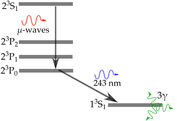
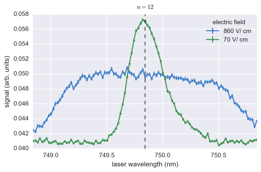
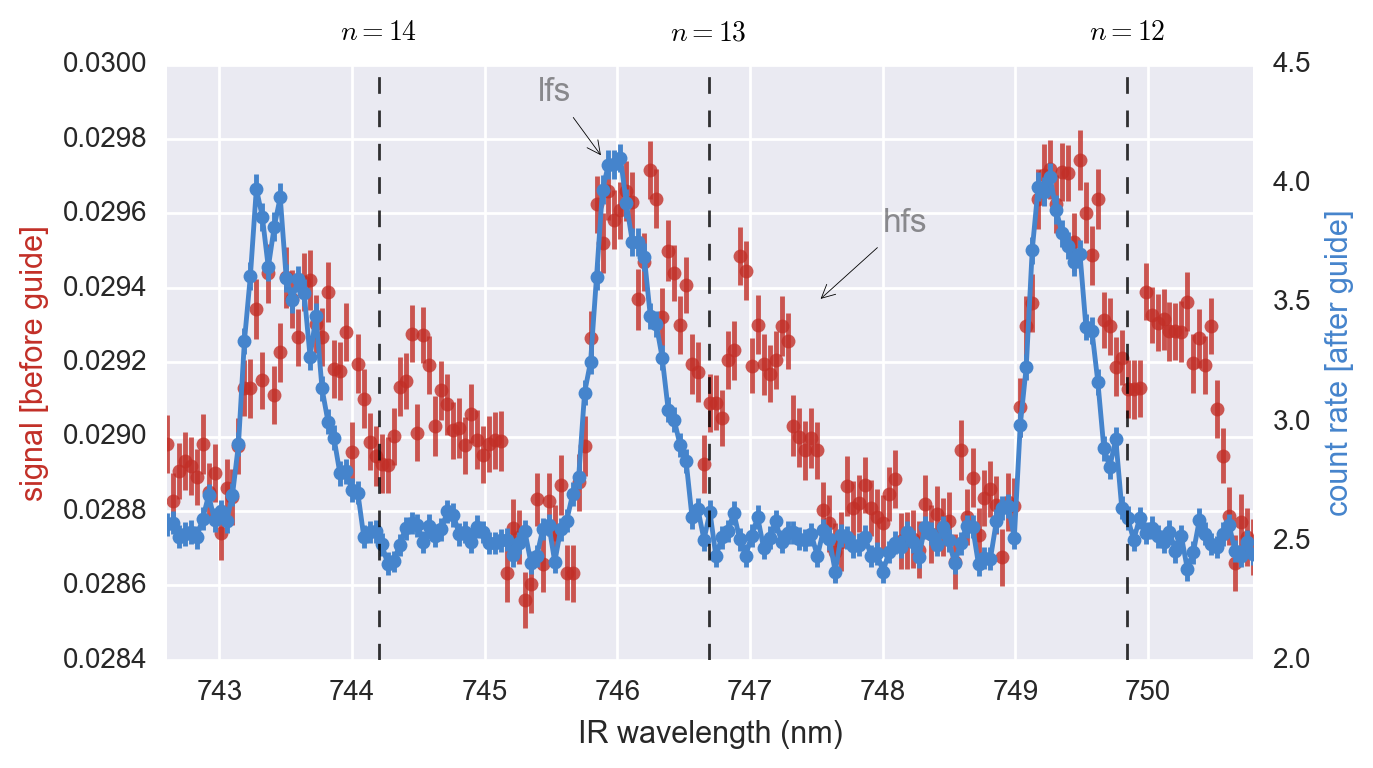
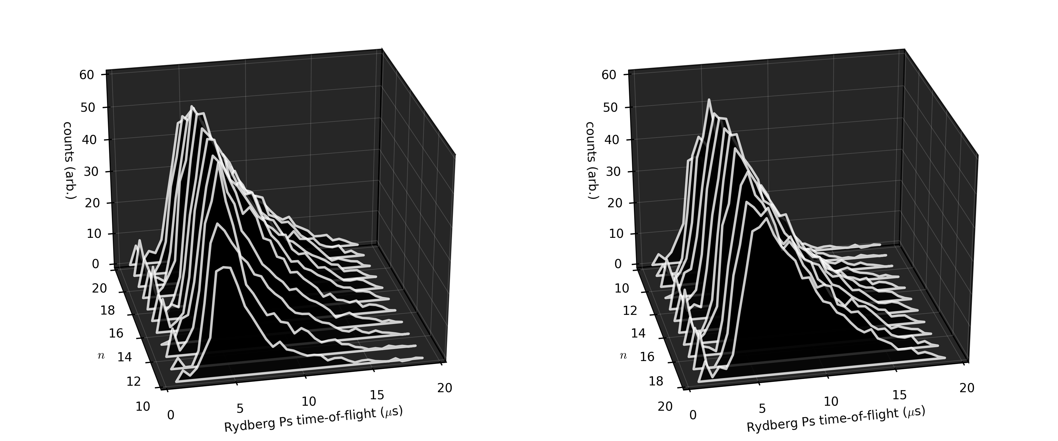
The figure above shows data taken by a detector set up for single-gamma-ray detection, approximately 12 cm away from the Ps production target, on the same experiment as described for the previous figure. It is clear from this data that the time-of-flight (TOF) to this detector is ~2 $\mu \mathrm{s}$ However, in this case it is clear that only the n = 19 state benefited from having the “switch on”, indicating that is the smallest-n state that this scheme is necessary for our current electric-field configuration.

Comparing the SSPALS and TOF figures it can be seen that even though the n = 18 SSPALS signal was changed drastically, the n = 18 TOF distribution remained the same, this is a clear example of how changes in the SSPALS spectrum discussed in the first figure are indicative of changes in atom distributions close to the Ps production region, but are not necessarily correlated to TOF distributions measured at different positions across the Ps flight paths

These methods will eventually lead to more accurate measurement of the lifetimes of higher n-states of Ps, and the possibility of using those states with higher electric dipole moments for future atom-optics experiments, such as Ps electrostatic lenses and Stark decelerators.

A guide to positronium

Published on July 31, 2016February 19, 2017 by de1lzLeave a comment

Positronium (Ps) is a hybrid of matter and antimatter. Made of just two particles – an electron and a positron – the atomic structure of Ps is similar to hydrogen. The ultimate aim of our experiments at UCL is to observe deflection of a Ps beam due to gravity, as nobody knows if antimatter falls up or down.

In this post, we outline how we recently managed to guide positronium using a quadrupole. Because the Ps atom doesn’t have a heavy nucleus, it’s extremely light and will typically move very, very quickly (~100 km/s). A refinement of the guiding techniques we used can, in principle, be applied to decelerate Ps atoms to speeds that are more suitable for studying gravity.

IMG_20160704_190341-01-01 — Point-of-view of a Ps atom entering a quadrupole guide

Before guiding positronium we have to create some. Positrons emitted from a radioisotope of sodium are trapped in a combination of electric and magnetic fields. They are ejected from the trap and implanted into a thin-film of mesoporous silica, where they bind to electrons to form Ps atoms; the network of tiny pores provides a way for these to get out and into vacuum.

The entire Ps distribution is emitted from the film in a time-window of just a few billionths of a second. This is well matched to our pulsed lasers, which we use to optically excite the atoms to Rydberg levels (high principal quantum number, n). If we didn’t excite the Ps then the electron-positron pairs would annihilate into gamma-ray photons in much less than a millionth of a second, and each would be unlikely to travel more than a few cm. However, in the excited states self-annihilation is almost completely suppressed and they can, therefore, travel much further.

Each Rydberg level contains many sublevels that have almost the same internal energy. This means that for a given n its sublevels can all be populated using a narrow range of laser wavelengths. But if an electric field is applied the sublevels are shifted. This so-called “Stark shift” comes from the electric dipole moment, i.e., the distribution of electric charge within the atom. The dipole is different for each sublevel and it can either be aligned or anti-aligned to the electric field. This results in a range of both positive and negative energy shifts, broadening the overall spectral line. Tuning the laser wavelength can now be used to select a particular sublevel. Or rather, to select a Rydberg-Stark state with a particular electric dipole moment. Stark broadening is demonstrated in the plot below. [For higher electric fields the individual Stark states can be resolved.]

linescan_fancy — Stark broadening of n=12 Ps in an electric field.

The Stark effect provides a way to manipulate the motion of neutral atoms using electric fields. As an atom moves between regions of different electric field strength its internal energy will shift according to its electric dipole moment. However, because the total energy must be conserved the kinetic energy will also change. Depending on whether the atom experiences a positive or negative Stark shift, increasing fields will either slow it down or speed it up. The Rydberg-Stark states can ,therefore, be broadly grouped as either low-field-seeking (LFS) or high-field-seeking (HFS). The force exerted by the electric field is much smaller than would be experienced by a charged particle. Nevertheless, this effect has been demonstrated as a useful tool for deflecting, guiding, decelerating, and trapping Rydberg atoms and polar molecules.

quadrupole_cartoon — Rydberg positronium source, lasers, gamma-ray detectors, and quadrupole guide.

A quadrupole is a device made from a square array of parallel rods. Positive voltage is applied to one diagonal pair and negative to the other. This creates an electric field that is zero along the centre but which is very large directly between neighbouring rods. The effect this has on atoms in LFS states is that when they drift away from the middle into the high fields they slow down, and eventually turn around and head back towards the centre, i.e., they are guided. On the other hand, atoms in HFS states are steered away from the low-field region and out to the side of the quadrupole.

Electric field strength and trajectory calculation for low-field-seeking (blue), high-field-seeking (red), and unaffected (green) Rydberg-Stark states of positronium in a quadrupole guide.

Using gamma-ray detectors at either end of a 40 cm long quadrupole we measured how many Rydberg Ps atoms entered and how many were transported through it. With the guide switched off some atoms from all states were transmitted. However, with the voltages switched on there was a five-fold increase in the number of low-field-seeking atoms getting through, whereas the high-field-seeking atoms could no longer pass at all.

total_fancy2 — The number of Rydberg Ps atoms entering (red) and passing all the way through (blue) the quadrupole guide.

A large part of why we chose to use positronium for our gravity studies is that it’s electrically neutral. As the electromagnetic force is so much stronger than gravity we, therefore, avoid otherwise overwhelming effects from stray electric fields. However, by exciting Ps to Rydberg-Stark states with large electric dipole moments we reintroduce the same problem. Nonetheless, it should be possible to exploit the LFS states to decelerate the atoms to low speeds, and then we can use microwaves to drive them to states with zero dipole moment. This will give us a cold Rydberg Ps distribution that is insensitive to electric fields and which can be used for gravitational deflection measurements.

Our article “Electrostatically guided Rydberg positronium” has been published in Physical Review Letters.

How long does Rydberg positronium live?

Published on April 29, 2016February 19, 2017 by de1lz1 Comment

Time-of-flight (TOF) is a simple but powerful technique that consists of accurately measuring the time it takes a particle/ atom/ ion/ molecule/ neutrino/ etc. to travel a known distance. This valuable tool has been used to characterise the kinetic energy distributions of an exhaustive range of sources, including positronium (Ps) [e.g. Howell et al, 1987], and is exploited widely in ion mass spectrometry.

Last year we published an article in which we described TOF measurements of ground-state (n=1) Ps atoms that were produced by implanting a short (5 ns) pulse of positrons into a porous silica film. Using pulsed lasers to photoionise (tear apart) the atoms at a range of well-defined positions, we were able to estimate the Ps velocity distribution, finding mean speeds on the order of 100 km/s. Extrapolating the measured flight paths back to the film’s surface indicated that the Ps took on average between 1 and 10 ns to escape the pores, depending on the depth to which the positrons were initially implanted.

When in the ground state and isolated in vacuum the electron and positron that make up a positronium atom will tend to annihilate each another in around 140 ns. Even with a speed of 100 km/s this means that Ps is unlikely to travel further than a couple of cm during its brief existence. Consequently, the photoionisation/ TOF measurements mentioned above were made within 6 mm of the silica film. However, instead of ionising the atoms, our lasers can be reconfigured to excite Ps to high-n Rydberg levels, and these typically live for a great deal longer. The increase in lifetime allows us to measure TOF spectra over much longer timescales (~10 µs) and distances (1.2 m).

TOF_schem

The image above depicts the layout of our TOF apparatus. Positrons from a Surko trap are guided by magnets to the silica film, wherein they bind to electrons and are remitted as Ps. Immediately after, ultraviolet and infra-red pulsed lasers drive the atoms to n=2 and then to Rydberg states. Unlike the positively charged positrons, the neutral Ps atoms are not deflected by the curved magnetic fields and are able to travel straight along the 1.2 m flight tube, eventually crashing into the end of the vacuum chamber. The annihilation gamma rays are there detected using an NaI scintillator and photomultipler tube (PMT), and the time delay between Ps production and gamma ray detection is digitally recorded.

unknown

The plots above show two different views of time-of-flight spectra accumulated with the infra-red laser tuned to address Rydberg levels in the range of n=10 to 20. The data shows that more Ps are detected at later times for the higher-n states than for lower-n states. This is easily explained by fluorescence, i.e., the decay of an excited-state atom via spontaneous emission of a photon. As the fluorescence lifetime increases with n, the lower-n states are more likely to decay to the ground state and then annihilate before reaching the end of the chamber, reducing the number of gamma rays seen by the NaI detector at later times. We estimate from this data that Ps atoms in n=10 fluoresce in about 3 µs, compared to roughly 30 µs for n=20.

This work brings us an important step closer to performing a positronium free-fall measurement. A flight path of at least ten meters will probably be required to observe gravitational deflection, so we still have some way to go.

This post is based on work discussed in our article:

Measurement of Rydberg positronium fluorescence lifetimes. A. Deller, A. M. Alonso, B. S. Cooper, S. D. Hogan, and D. B. Cassidy. Phys. Rev. A 93, 062513 (2016)DOI:10.1103/PhysRevA.93.062513.

Controlling Positronium Annihilation with Electric Fields

Published on October 29, 2015February 19, 2017 by AlbertoMAlonsoUCL1 Comment

To produce Rydberg (highly-excited) states of positronium we use a multi-photon $1 ^3S \rightarrow 2 ^3P \rightarrow nS/nD$ excitation scheme [1]. These high- $n$ Ps atoms are long-lived and could potentially be used for (anti)-gravity measurements, however, the intermediate state ( $n=2$ ) has interesting properties of it’s own, as described in our latest article (Phys. Rev. Lett. 115, 183401 ).

Unlike regular atoms, Ps has the peculiar feature that it can self-annihilate into gamma-rays. The amount of overlap between the positron and electron wave functions depends on the particular state the atom is in, and this determines how long before self-annihilation occurs (characterised by the average annihilation lifetime). The quantum spin ( $s=1/2$ ) of the electron and positron can combine in positronium to either cancel ( $S=0$ ) or sum ( $S=1$ ), depending on the relative alignment between the two components. In the former case (para-Ps) the atom has a very short ground-state lifetime of just 125 ps, whereas in the latter case (ortho-Ps) the atom lives in the $n=1$ state for an average of 142 ns (this may not sound very long but it’s actually plenty of time to do spectroscopy with pulsed lasers).

We produce $n=1$ ortho-Ps ( $1^3S_1$ ) atoms then excite these using 243 nm laser light from our UV laser. The electronic dipole transition selection rules (principally, $\Delta S= 0$ and $\Delta \ell = \pm 1$ ) dictate that this single-photon transition drives the atoms to the $n = 2$ , $\ell= 1$ , $S= 1$ state ( $2 ^3P_J$ ). For historical reasons the orbital angular momentum is written here as $S$ ( $\ell= 0$ ) and $P$ ( $\ell= 1$ ).

The fluorescence lifetime of an excited atom is the time it takes, on average, to spontaneously emit a photon and decay to a lower energy state. All of the $n=2, \ell = 1$ states have a fluorescence lifetime of 3.19 ns, and an annihilation lifetime of over 100 $\mu$ s (practically infinite compared to the time-scale of our measurements, i.e., $2^3P$ states don’t annihilate directly, but can decay to a different state then annihilate). The $n=2, \ell = 0$ ortho and para states have annihilation lifetimes of 1136 ns and 1 ns, and they both fluoresce with a lifetime of $\simeq$ 0.24 s ( $\approx \infty$ ). The bottom line here is that there are a wide range of fluorescence and annihilation lifetimes for the various possible sub-states in the $n=1$ and $n=2$ manifolds.

In a magnetic field the short-lived $S=0$ and longer-lived $S=1$ states (with the same $\ell$ ) are mixed together (Zeeeman mixing). Similarly, an electric field mixes states with different $\ell$ (but the same $S$ ) (Stark mixing). By exciting Ps to $n = 2$ in a weak magnetic field then varying an electric field, we can tailor the extent of this mixing to increase or decrease the overall lifetime. This technique can be used to greatly increase the excitation efficiency to another state, since the losses due to annihilation can be reduced. Conversely, increasing the annihilation rate can be used as an efficient way to detect excitation.

The polarization orientation of the UV excitation laser gives us some control over which $M_J$ states are subsequently populated. More specifically, if the laser polarization is parallel to the applied magnetic field then only $\Delta M_J=0$ transitions are allowed, whereas if the polarization is perpendicular to it then $\Delta M_J$ must change by $\pm 1$ .

Below is a calculation of how the $n=2$ energy levels are shifted by an electric field, in zero magnetic field (red) and in a magnetic field of 13 mT (blue). Note the avoided crossing at 585 V/ cm in the 13 mT case.
StarkmapFig So what can we actually measure? In most cases, laser excitation makes it more likely for ground state ortho-Ps to ultimately end up in the short-lived para-Ps state, thus applying the laser causes an increase in the annihilation gamma ray flux at early times. This change can be observed and quantified using the parameter $S$ (higher values means more gamma rays were detected compared to a measurement made without the laser). This is plotted below for various electric field strengths, and with the laser polarised either parallel (red) or perpendicular (green) to the magnetic field. In both cases, the avoided crossing gives a sharp increase in annihilation rate (see the “ears” in both plots), whilst higher electric fields either reduce or increase the signal, depending on which $M_J$ states the laser initially populates.

Quenching

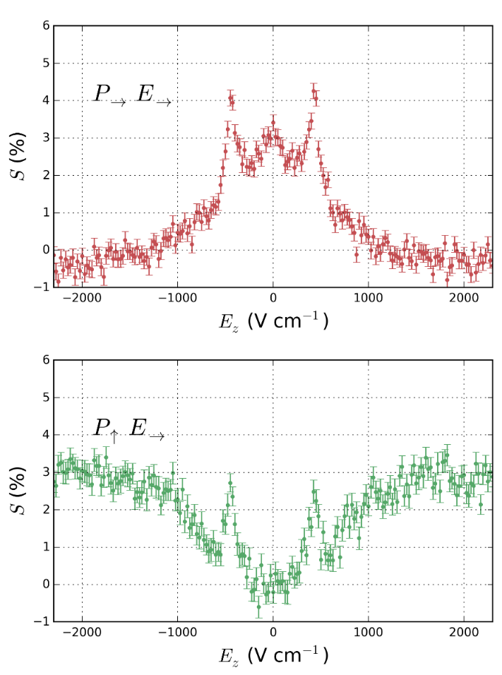
Notice that when the laser polarisation is aligned parallel to the magnetic field (red), very high electric fields lead to negative $S$ values. This means that the lifetime of the Ps becomes longer than 142 ns (the ground-state ortho-Ps lifetime) if the laser is applied. This is due to the fact that in this field configuration there is significant mixing into the long lived $2^3S_1$ state. This could be used to produce an ensemble of pure $2^3S_1$ states, by exciting Ps in this high field and then extracting the excited state into a region of zero field. These pure states could be exploited for $n=2$ microwave spectroscopy [3].

[1] Selective Production of Rydberg-Stark States of Positronium. T. E. Wall, A. M. Alonso, B. S. Cooper, A. Deller, S. D. Hogan, and D. B. Cassidy, Phys. Rev. Lett. 114, 173001 (2015) DOI:10.1103/PhysRevLett.114.173001.

[2] Controlling Positronium Annihilation with Electric Fields. A. M. Alonso, B. S. Cooper, A. Deller, S. D. Hogan, D. B. Cassidy, Phys. Rev. Lett. 115, 183401 (2015) DOI:10.1103/PhysRevLett.115.183401.

[3] Fine-Structure Measurement in the First Excited State of Positronium. A. P. Mills, S. Berko, and K. F. Canter, Phys. Rev. Lett. 34, 1541 (1975) DOI:/10.1103/PhysRevLett.34.1541.

Time-resolved Doppler spectroscopy

Published on January 30, 2015February 19, 2017 by AlbertoMAlonsoUCL1 Comment

Positronium atoms created by implanting positrons into porous silica initially have ~ 1 eV kinetic energy, but subsequently cool by colliding with the inner surfaces of the porous network. The longer spent inside the pores before being emitted to vacuum, the closer the Ps can get to thermalising with the bulk (i.e. room temperature, ~ 25 meV).

Once the positronium atoms make it out of the pores and into vacuum we can excite them using a 243 nm (UV) pulsed laser to n = 2, then ionize these with a 532~nm (green) laser. The amount of positrons resonantly ionised can be measured using SSPALS as the UV wavelength is slowly varied. This gives us the 1s2p Doppler-width, from which we estimate the Ps energy. The delay between implanting positrons and firing the 6 ns laser pulse was varied to try and see how the width changes when hitting the Ps cloud at different times.

In the 3D plot above we see that at earlier times the Doppler width is broader than later on. This is because Ps atoms that spend longer inside the silica have more collisions with the pores and therefore cool down further (narrowing the distribution at later times), mixed up with the simple fact that the fastest atoms reach the laser interaction region quickest, and pass through it more quickly too!

Rydberg Positronium and Stark broadening

Published on November 30, 2014February 19, 2017 by AlbertoMAlonsoUCL1 Comment

We have recently produced Rydberg positronium atoms in a two step excitation process, using 243 nm light from our broad band pulsed dye laser to excite 2P states, as in our previous Ps spectroscopy measurements. Then, instead of photoionizing with 532 nm light, we used ~ 750 nm light to excite 2p-nd transitions. This process is shown in the energy level diagram below, you can also see a photograph of the green light produced by our Nd:YAG laser pumping the infra red laser.

Once the Ps atoms have been excited to a Rydberg state, their lifetime is greatly increased, and they only annihilate once they collide with the vacuum chamber. This leads to a reduced delayed fraction in our positronium SSPALS signal, since there are less gamma ray events occurring on our delayed detection time (to read more about how we detect Ps, read here). This can be seen in our data below where we excited Ps atoms to n = 11.

When atoms are subjected to a high electric field different states are separated and shifted leading to an overall broadening of the spectral line, this effect is known as Stark broadening, the mixing and shifting of the states is proportional to the strength of the electric field being applied. We are able to observe this effect by varying the voltage applied to our porous silica target from which Ps atoms are produced, and therefore changing the electric field that the Ps atoms are subjected to. As the voltage is increased, the broadening grows with the eclectic field, thus producing a signal over a wider range of infra red wavelengths, this is shown in the figure above where we plot the delayed fraction over a range of 5.6 nm, changing the voltage applied to our target from from 1 kV to 2 kV and 3 kV.