Ethics in research is something everyone is expected to understand and respect, from beginning students to established professors. However, very rarely are such things discussed formally. In effect one is expected to simply know all about these matters by appealing to “common sense” and also to the examples set by mentors. This is not an ideal situation, as is evidenced by numerous high profile cases of scientific misconduct. The purpose of this post is to briefly mention some important aspects of ethical research practices, mostly to encourage further thought in students before they have a chance to influenced by whatever environment in which they are working.
In some cases “misconduct” is easy to spot, and is then (usually) universally condemned. For example, making up or manipulating data is something we all know is wrong and for which there can never be a legitimate defense. At the same time, some students might see nothing wrong in leaving off a few outlier data points that clearly do not fit with others, or in failing to refer to some earlier paper. It is not always necessarily obvious what the right (that is to say, ethical) thing to do might be. What harm is there, after all, in putting an esteemed professor as a co-author on a paper, even though they have provided no real contribution? (Incidentally, merely providing lab space, equipment or even funding doesn’t, or shouldn’t, count as such). Well, there is harm in gift authorship; it devalues the work put in by the real authors, and makes it possible for a certain level of authority to guarantee future (perhaps unwarranted) success. And does it really matter if an extreme outlier is left off of an otherwise nice looking graph? The answer is yes, absolutely.
At the heart of most unethical behavior in science, or misconduct, is the nature of truth, and the much revered “scientific method”. Never mind that there is no such thing, or that the way science is actually done is not even remotely similar to the romantic notions so often associated with this very human activity. Nevertheless, there is a very strong element of trust implicit in the scientific endeavor. When we read scientific papers we have no choice but to assume that the experiments were carried out as reported, and that the data presented is what was actually observed. The entire scientific enterprise depends on this kind of trust; if we had to try and sort through potentially fraudulent reports we would never get anywhere. For this reason, trust in science is extremely important, and one could say that, regardless of any mechanisms of self correction that might exist in science, and the concomitant inevitability of discovery of fraud, we are almost compelled to trust scientists if we wish science to be done in a reasonable manner[a]. By the same token, those scientists who choose to betray this trust pollute not only their own research (and personal character), but all science. The enormity of this offense should not be understated. In particular, students should be aware of the fact that being a dishonest scientist is oxymoronic.
What is misconduct? A formal definition of scientific misconduct of the sort that would be necessary in legal action is an extremely difficult thing to produce. There have been many attempts, most of which are centered on the ideas of FFP: that is, fraud, falsification and plagiarism. These are things that we can easily understand and, most of the time, identify when they arise. However, things can (and invariably do) get complicated in real world situations, especially when people try to gauge intention, or when the available information is incomplete.
A definition of scientific misconduct, as it pertains to conducting experiments or observations to generate data, was given by Charles Babbage (Babbage 1830) that still has a great deal of relevance today. Babbage is perhaps best known for his “difference engine”, a mechanical computer he built to take the drudgery out of performing certain calculations. He was a well-respected scientist working in many areas, Professor of physics at Cambridge University and a fellow of the Royal society. His litany of offences, which is frequently cited in discussions of scientific misconduct, was categorized into four classes.
Babbage’s taxonomy of fraud:
1.) Hoaxing is not fraud in the usual sense, in that it is generally intended as a joke, or to embarrass or attack individuals (or institutions). A hoax is more like a prank than an attempt to benefit the hoaxster in the scientific realm; it is not often that a hoax remains undisclosed for a long time. Hoaxes are not generally intended to promote the perpetrator, who will prefer to remain anonymous, (at least until the jig is up). A Hoax is far more likely to involve someone dressing up as Bigfoot, or lowering a Frisbee outside a window on a fishing line than fabricating IV curves for electronic devices that have never been built.
A famous and amusing example is the so-called Sokal hoax (Sokal 1996). In 1996 a physicist from New York University submitted a paper to the journal “Social Text”. This journal publishes work in the field of “postmodernism” or cultural studies, an area in which there had been many critiques of science based on unscientific criteria. For example, the idea that scientific objectivity was a myth, and that certain cultural elements (e.g., “male privilege” or western societal norms) are determining factors in the underlying nature of scientific discovery. This attitude vexed many physicists, leading to the so-called “science wars” (Ross 1996), and was the impetus for Sokal’s hoax. The paper he submitted to Social Text was entitled “Transgressing the Boundaries: Towards a Transformative Hermeneutics of Quantum Gravity”. This article was deliberately written in impenetrable language (as was often the case in articles in Social text, and other similar publications) but was in fact pure nonsense (as was also often the case in articles in Social text and other similar publications). The paper was designed with the intention of impressing the editors, not only with the stature of the author (Sokal was then a respected physicist, and seems at the time of writing, some 16 years later, still to be one) but also by appealing to their ideological positions. Sokal revealed the hoax immediately after his paper was published; he never had any intention of allowing it to stand, but rather wanted to critique the journal. As one might expect, a long series of arguments arose from this hoax, although the main effect was to tempt more actual scientists into commenting on the “science wars” that were already occurring. In this sense Sokal may have done more harm than good with his hoax, as the inclusion of scientists in the “debate” served only to legitimize what had before been largely the province of people with no training in, or, frequently, understanding of, science.
2.) Forging is just what it sounds like, simply inventing data and passing it off as real. Of course, one might do the same in a hoax, but the forger seeks not to fool his audience for a while, later to reveal the hoax for his or her own purposes, but to permanently perpetrate the deception. The forger will imitate data and make it look as real as possible, and then steadfastly stick to their claim that it is indeed genuine. Often such claims can stand up to scrutiny even once the forging has been exposed, since if it is done well the bogus data is in no way obviously so. This unfortunate fact means that we cannot know for sure how much forging is really going on. However, the forger does not have any new information and so cannot genuinely advance science. They may be able to appear to be doing so, by confirming theoretical predictions, for example, but such predictions are not always correct. Nevertheless, the forger must have a good knowledge of their field, and enough understanding of what is expected to be able to produce convincing data out of thin air. If one were to do this then, on rare occasions, it is even possible that one might guess at some reality, later proved, and really get away with it. However, the fleeting glory of a major discovery seems to be somewhat addictive to those so inclined, and some famous forgers have started out small, only to allow themselves to be tempted into such outrageous claims that from the outside it seems as though they wanted to get caught.
A well known case in which exactly this happened is the “Schön affair”, which has been covered in detail in the excellent book “plastic fantastic” (Reich 2009). Hendrik Schön was a young and, apparently, brilliant young physicist employed at Bell Labs in the early 2000’s. His area of expertise was in organic semiconductors, which held (and continue to hold) great promise for the production of cheap and small electronic devices. Schön published a large number of papers in the most high profile journals (including many in Science and Nature) that purported to show organic crystals exhibiting remarkable electronic properties, such as superconductivity, the fractional quantum hall-effect, lasing, single molecule switches and so on. At one point he was publishing almost one paper per week, which is impressive just from the point of view of being able to write at such a rate; most scientists will probably spend one or two months just writing a paper, never mind the time taken to actually get the data or design and build an experiment. Before the fraud was exposed one professor at Princeton University[b], who had been asked to recommend Schön for a faculty position, refused to do so, and stated that he should be investigated for misconduct based solely on his extreme publication rate (Reich 2006).
Schön’s incredible success seemed to be predicated on his unique ability to grow high quality crystals (he was described on one occasion as having “magic hands”). This skill eluded other researchers, and nobody was able to reproduce any of Schön’s results. As he piled spectacular discovery upon spectacular discovery, suspicion grew. Eventually it was noticed that in some of his published data Schön had used the same curves, right down to the noise, to represent completely distinct phenomena, in completely different samples (that, in fact, had never really existed). After trying to claim that this was simply an accident, that he had just mislabeled some graphs and used the wrong data, more anomalies were revealed. The management at Bell labs started an investigation and Schön continued to make excuses, stating (amazingly, considering the quality of the real scientists that worked at this world leading institution) that he had not kept records in a notebook, and that he had erased his primary data to make space on his computer’s hard drive[c]!
None of these excuses were convincing, and indeed such poor research techniques should themselves probably be grounds for dismissal, even in the absence of fraud. Fraud was not absent, however, it was prevalent, and on a truly astounding scale. Schön had invented all of his data, wholesale, had never grown any high quality crystals, and had lied to many of his colleagues, at Bell labs and elsewhere. He was fired, and his PhD was revoked by Konstantz university in Germany for “dishonorable conduct”. There was no suggestion that the rather pedestrian research Schön had completed for his doctorate was fraudulent, but his actual fraud was so egregious that his university felt that he had dishonored not just himself and their institution, but science itself, and as such did not deserve his doctorate.
It seems obvious in retrospect that Schön could never have expected to get away with his forging indefinitely. Even if he had been a more careful forger, and had made up distinct data sets for all of his papers, the failure of others to reproduce his work would have eventually revealed his conduct. Even before he was exposed, pressure was mounting on Schön to explain to other scientists how he made his crystals, or to provide them with samples. He had numerous, and very well respected, co-authors who themselves were becoming nervous about the increasingly frustrated complaints from the other groups unable to replicate his experiments. It was only a matter of time before it all came out, regardless of the manifestly fake published data.
This unfortunate affair raises some interesting questions about misconduct in science. For example, Schön’s many co-authors seem to have failed in their responsibilities. Although they were found innocent of any actual complicity in the fraud, as co-authors on so many, and on such astounding, papers, it seems clear that they should have paid more attention. Some of the co-authors were highly accomplished scientists, while Schön himself was relatively junior, which only compounds the apparent lack of oversight. Indeed, it is likely that the pressure of working for such distinguished people, and at such a well-respected institution as Bell Labs, was what first tempted Schön into his shameful acts.
No doubt winning numerous prizes, being offered tenured positions at an Ivy League school (Princeton; not bad if you can get an offer) and generally being perceived as the new boy-wonder physicist played a role in the seemingly insane need to keep claiming ever more incredible results. It is hard to escape the conclusion that some sort of mental breakdown contributed to this folly. However, another pathological element was also likely at play, which is that Schön was sure that his speculations would eventually be borne out by other researchers.
If this had actually happened, and if he had not been a poor forger (or, perhaps, an overworked forger, with barely enough time to invent the required data), he might have enjoyed many years of continued prosperity. As it happens, some of the fake results published by Schön have in fact been shown to be roughly correct; sometimes the theorists guess right. Ultimately though, forging will usually be found out, and the more that is forged the faster this will happen. The only way to forge and get away with it is to know in advance what nature will do, and if you know that the forging is redundant[d].
3.) Trimming is the practice of throwing away some data points that seem to be at odds with the rest of the measurements, or at least are not as close to the “right” answer as expected. In this case the misconduct is primarily designed to make the experimenter seem more competent, although actually a poor knowledge of statistics might mean that it has the opposite effect; outliers sometimes seem out of place, but, to those who have a good knowledge of statistics, their absence may be quite suspicious. Because it can seem so innocuous, trimming is probably much more common than forging. When he invents data from nothing, the forger has already committed himself to what he must surely know is an immoral and heinous action; whatever justification he might employ towards this action cannot shield him from such knowledge. The trimmer, on the other hand, might feel that his scientific integrity is unaffected, and that all he is doing is making his true data a little more presentable; so as to better explain his truth. A trimmer who believes this is wrong may well be less offensive than the forger, but his actions are still unconscionable, will still constitute a fraud, and may equally well pervert the scientific record, even when the essential facts of the measurement remain. For example, by trimming a data set to look “nicer” you might significantly alter the statistical significance of some slight effect. Indeed, in this way you can create a non-existent effect, or destroy evidence for a real one; without the truth of nature’s reference there is no way to know the difference.
The trimmer has a great advantage over the forger, insofar as he is not trying to second guess nature, but rather obtains the answer from nature in the form of his primary measurements, and then attempts to make his methodology in so doing appear to be “better” than it really was. The trimmed data, therefore, will likely not give a very different answer than the untrimmed set, but will seem to have been obtained with greater skill and precision.
There are no well known examples of trimming because, by its very nature, it is hard to detect. Who will know if some few data points are omitted from an otherwise legitimate data set? What indicators might allow us to distinguish a careful experimenter from a carefree trimmer? Even Newton has been accused of trimming some of his observations of lunar orbits to obtain better agreement with his theory of gravitation (Westfell 1996). Objectively, even for the amoral, trimming is quite pointless when one considers that, if found out, the trimmer will suffer substantial damage to his reputation, whereas even if it is not found out, the advantage to that reputation is slight.
4.) Cooking refers to selecting data that agrees with the hypothesis you are trying to prove and rejecting other data, that may be equally valid, but that doesn’t. In other words, cherry picking. This is similar to trimming inasmuch as it is selecting from real data (i.e., not forged), but with no real justification for doing so, other than ones own presupposition about what the “right” answer is. It differs from trimming, for the cook will take lots of data and then select those that serve his purpose, while the trimmer will simply make the best out of whatever data he has. This is lying, just as forging, but with the limitation that nature herself has at least suggested which lies to tell.
Cooking also carries with it an ill defined aspect of experimental science, that of the “art” of the experimentalist. It is certainly true to say that experimental physics (and no doubt other branches of science too) contains some element of artistry. Setting up a complicated apparatus and making it work is an underappreciated skill, but a crucial one. When taking data with a temperamental system it is routine to throw some of it out, but only if one can justify doing so it in terms of the operation of the device. Almost all experiments include some tuning up time in which data are neglected because of various experimental problems. However, once all of these problems have been ironed out and the data collection begins “for real” one has to be very careful about excluding any measurements. If some obvious problems attend (a power supply failed, a necessary cable was unplugged, batboy was seen chewing on the beamline, whatever it may be) then there is no moral difficulty associated with ditching the resulting data. When this sort of thing happens (and it will), the best thing to do is throw out all of the data and start again.
The situation gets more complicated if an intermittent problem arises during an experiment that affects only some of the data. In that case you might want to select the “good” data and get rid of the “bad”. Unfortunately all of the resulting data will then be “ugly”. This is not a good idea because it borders on cooking. It is much better to throw away all potentially suspect data and start again. In data collection, as in life, even the appearance of impropriety can be a problem, regardless of if propriety has in fact been maintained. It may be the case that there is an easy way to identify data points that are problematic (for example, the detector output voltage might be zero sometimes and normal at others), but there will remain the possibility that the “good” data is also affected by the underlying experimental problem leading to “bad” data, but in a less obvious manner. The best thing to do in this situation will depend on many factors. It is not always possible to repeat experiments; you might have a high confidence in some data because of the exact nature of your apparatus and so on. Even so, “when in doubt, throw it out” is the safest policy.
Cooking is a little like forging, but with an insurance policy. That is, since the data is not completely made up there is a better chance that it does really correspond to nature, and therefore you will not be found out later because you are (sort of) measuring something real. This is not necessarily the case, however, and will depend on the skill of the cook. By selecting data from a large array it is usually possible to produce “support” for any conclusion one wants, and as a result the cook who seeks to prove an incorrect hypothesis loses his edge over the forger.
A well known case illustrates that it is not so simple to decouple experimental methodology with cookery. Robert Millikan is well known for his oil drop experiment in which he was able to obtain a very accurate value for the charge on an electron, work for which he was awarded the Nobel Prize. This work has been the subject of some controversy, however, since Historian of Science Gerald Holton [Holton 1978] went through Millikan’s notebooks and revealed that not all of the available data had been used, even though Millikan specifically said that it had. Since then there have been numerous arguments about whether the selection of data was simply the shrewd action of an expert experimentalist, or one of dishonest cooking. As discussed by numerous authors [e.g., Segerstråle, 1995] it is neither one nor the other, and the situation is more nuanced. The reality is that his answer was remarkably accurate, as we now know. The question then is did Millikan know what to expect? If he did not then accusations of cooking seem unfounded, since he would have had to know what he was trying to “demonstrate”. If he got the right answer without knowing it in advance, he must have been doing good science, right? WRONG! If Millikan was cooking (or even doing a little trimming) and he somehow got the right answer this does not in any way mitigate the action. Since we cannot say whether he really did do any cooking or not, one might believe that getting the right answer implies that he was being honest; as it turns out, he would have obtained an even more accurate answer if he had used all of his data (Judson 2004).
Furthermore, the question of whether Millikan already knew the “right” answer is meaningless. The right answer is the one we get from an experiment, and we only know it to the extent that we can trust the experiment. An army of theoreticians can be (have been, perhaps now are) wrong. Dirac predicted that the electron g factor would be exactly 2, and it almost is. Knowing only this, the cook or trimmer might be sorely tempted to nudge the data to be exactly 2.0000 and not 2.0023, but that would be a terrible mistake, one that would miss out on a fantastic discovery. One can only hope that somewhere in the world there is at least one cook who allowed a Nobel Prize (or some major discovery) to slip through his dishonest fingers, and cannot even tell anyone how close he came. Did Millikan knowingly select data to make his measurements look more accurate? There is no way to know for sure.
Pathological science is a term coined by Irving Langmuir, the well known physicist. He defined this as science in which the observed effects are barely detectable, and the signals cannot be increased, but are nevertheless claimed to be made with great accuracy; pathological science also frequently involves unusual theories that seem to contradict what is known (Langmuir 1968). However, pathological science is not usually an act of deliberate fraud, but rather one of self delusion. This is why the effect in question is always at the very limit of what can be detected, for in this case all kinds of mechanisms can be used (even subconsciously) to convince one that the effect really is real. In this context, then, it is worth asking, does the cook necessarily know what he is doing? That is, when one wishes to believe something so very strongly, perhaps it becomes possible to fool ones own brain! This kind of self delusion is more common than you might think, and happens in everyday life all the time. Although we cannot directly choose what we believe is true, when we don’t know one way or the other, our psychology makes it easy for us to accept the explanation that causes the least internal conflict (also known as cognitive dissonance).
When a researcher is so deluded as to engage in pathological science, it is difficult to categorize this activity as one of misconduct. The forger has to know what he is doing. The trimmer or cook generally tries to make his data look the way he wants, but if he does so without real justification then it is wrong. By making justifications that seem reasonable but are not, one could conceivably fool oneself into thinking that there was nothing improper about cooking or trimming. Certainly, this will sometimes really be the case, which only makes it easier to come up with such justifications.
In many regards the pathological scientist is not so different from one who is simply wrong. The most famous example of this might be the cold fusion debacle (Seife 2009). Pons and Fleischmann claimed to see evidence for room temperature fusion reactions and amazed the world with their press conferences (not so much with their data). Later their fusion claims turned out to be false, as proved by Kelvin Lynn, Mario Gai and others (Gai et al 1989). However, the effect they said they saw was also observed by some other researchers, and as a result many reasons were promulgated as to why one experiment might see it and another might not. Then, when it was pointed out that there ought to be neutron emission if there was fusion, and no neutrons were observed, it became necessary to modify the theory so as to make the neutrons disappear. This was classic pathological science, hitting just about every symptom laid out by Langmuir.
Plagiarism was not explicitly discussed by Babbage but does feature prominently in modern definitions of misconduct. Directly copying other peoples work is relatively rare for professional scientists, perhaps because it is so likely to be discovered. There have been some cases in which people have taken papers published in relatively obscure journals and submitted them, almost verbatim, to other, even more obscure, journals. Since only relatively unknown work is susceptible to this sort of plagiarism it does little damage to the scientific record, but is no less of an egregious act for this. Certainly the psychology of the “scientist” who would engage in such actions is no less damaged than that of a Schön.
In one case a plagiarist, Andrzej Jendryczko, tried to pass of the work of others as his own by translating it (from English, mostly) into Polish, and then publishing direct copies in specialized Polish medical journals under his own name (E.g., Judson 2004). This may have seemed like a safe strategy, but a well read Polish-American physician had no trouble tracking down all the offending papers using the internet. Indeed, wholesale plagiarism is now very easy to uncover via online databases and a multitude of specialized software applications. For the student, plagiarism should seem like a very risky business indeed. With minimal effort it can be found out, and no matter how clever the potential plagiarist might be, Google is usually able to do better with sheer force of computing power and some very sophisticated search algorithms. As is often the case, this sort of cheating does not even pass a rudimentary cost-benefit analysis[e]. It is another inverse to Pascal’s wager (the idea that it is better to believe in God than not, just because the eternity of paradise always beats any temporary secular position) inasmuch as the actual gain attending ripping off some (necessarily) obscure article found online is virtually nil, whereas exposure as a fraud for doing this will contaminate everything you have ever done, or will ever do, in science. How can this ever be worth even considering?
Plagiarism is not as simple as copying the work of others; providing incomplete references in a paper could be construed as a form of plagiarism, insofar as one is not providing the appropriate background, thereby perhaps implying more originality than really exists. References are a very important part of scientific publishing, and not just because it is important to give due respect to the work that you might be building upon. A well referenced paper not only shows that you have a good understanding and knowledge of your field, but will also make it possible for the reader to properly follow the research trail, which puts everything in context and helps enormously in understanding the work[f].
Stealing the ideas of others, if not their words, is also, of course, a form of plagiarism. This is harder to prove, which may be why it is something most often discussed in the context of grant proposals. This forms a rather unfortunate set of circumstances in which a researcher finds himself having to submit his very best ideas to some agency (in the hope of obtaining funding), which are promptly sent directly to his most immediate competitors for evaluation! After all, it is your competition who are best placed to evaluate you work. In most cases, if an obvious conflict exists, it is possible to specify individuals who should not be consulted as referees, although this is more common in the publication of papers than it is in proposal reviews. For researchers in niche fields, in which there may not be as much rivalry, this is not going to be a common problem. For researchers in direct competition, however, things might not be so nice. There have in fact been some well publicized examples of this sort of plagiarism, but it is probably not very common because grant proposals don’t often contain ideas that have not been discussed, to some degree, in the literature, and in those rare cases when this isn’t so, it is probably going to be obvious if such an idea is purloined. Also, let us not forget, most scientists are really not so unscrupulous. Thus, for this to happen you’d need an unlikely confluence of an unusually good idea sent to an abnormally unprincipled referee who happened to be in just the right position to make use of it.
References & Further Reading
Misconduct in science is a vast area of study, and the brief synopsis we have given here is just the tip of the iceberg. The use of Babbage’s taxonomy is commonplace, and in depth discussions of every aspect of this can be found in many books. The following is small selection. The book by Judson is particularly recommended as it is fairly recent and goes into just the right amount of detail in some important case studies.
https://retractionwatch.com/
Judson H. F. (2004). The Great Betrayal: Fraud in Science, Houghton Mifflin Harcourt.
Alfredo K and Hart H, “The University and the Responsible Conduct of Research: Who is Responsible for What?” Science and Engineering Ethics, (2010).
Sterken, C., “Writing a Scientific Paper III. Ethical Aspects”, EAS Publications Series 50, 173 (2011)
Reich, E. S. (2009). Plastic Fantastic: How the Biggest Fraud in Physics Shook the Scientific World, Palgrave Macmillan.
Broad, W. and Wade, N. (1983). Betrayers of the Truth: Fraud and deceit in the halls of science, Simon & Schuster.
Babbage C. (1830) Reflections on the Decline of Science in England, August M. Kelley, New York (1970).
Holton G. (1978) Subelectrons, presuppositions and the Millikan-Ehrenhaft dispute, In: Holton G., ed., The Scientific Imagination, Cambridge University Press, Cambridge, UK.
Langmuir I. (1989) Pathological science, Physics Today 42: 36–48. Reprinted from the original in General Electric Research and Development Center Report 86-C-035, April 1968
Ross, Andrew, ed. (1996). Science Wars. Duke University Press.
Segerstråle, U. (1995). Good to the last drop? Millikan stories as “canned” pedagogy, Science and Engineering Ethics 1, 197.
Sokal, A., D. and Bricmont, J. (1998). Fashionable Nonsense: Postmodern Intellectuals’ Abuse of Science. Picador USA: New York.
Westfall, R., S. (1994). The Life of Isaac Newton. Cambridge University Press.
Seife, C. (2009). Sun in a Bottle: The Strange History of Fusion and the Science of Wishful Thinking, Penguin Books.
Gai, M. et al., (1989). Upper limits on neutron and gamma ray emission from cold fusion, Nature 340, 29.
Footnotes
[a] What is this reasonable manner? We just mean that if one cannot trust scientific reports to be honest representations of real work undertaken in good faith, then standing on the shoulders of our colleagues (who may or may not be giants) becomes pointless, everything has to be independently verified, and the whole scientific endeavor becomes exponentially more difficult.
[b] Reich’s book does not name the professor in question, but clearly he or she had a good grasp on how much can be done, even by a highly motivated genius.
[c] This is a particularly ludicrous claim since to a scientist experimental data is a highly valuable commodity, whereas disc space is trivially available: the idea that one would delete primary data just to make space on a hard drive is like burning down one’s house in order to have a bigger garden.
[d] Another way to increase your chances of getting away with forgery is to fake data that nobody cares about. However, this obviously has an even less attractive cost-benefit ratio.
[e] We obviously do not mean to suggest that some clever form of plagiarism that can escape detection does pass a cost-benefit analysis, and is therefore a good idea: the uncounted cost in any fraud, even a trivial one, is the absolute destruction of one’s scientific integrity. We just mean that this sort of thing, which is never worthwhile, is even more foolish if there isn’t some actual (albeit temporary) advantage.
[f] On a more mundane level, a referee who has not been cited, but should have been, is less likely to look favorably upon your paper than he or she might otherwise have done. This also applies to grant proposals, so it is in your own interests to make sure your references are correct and proper.


 .
.


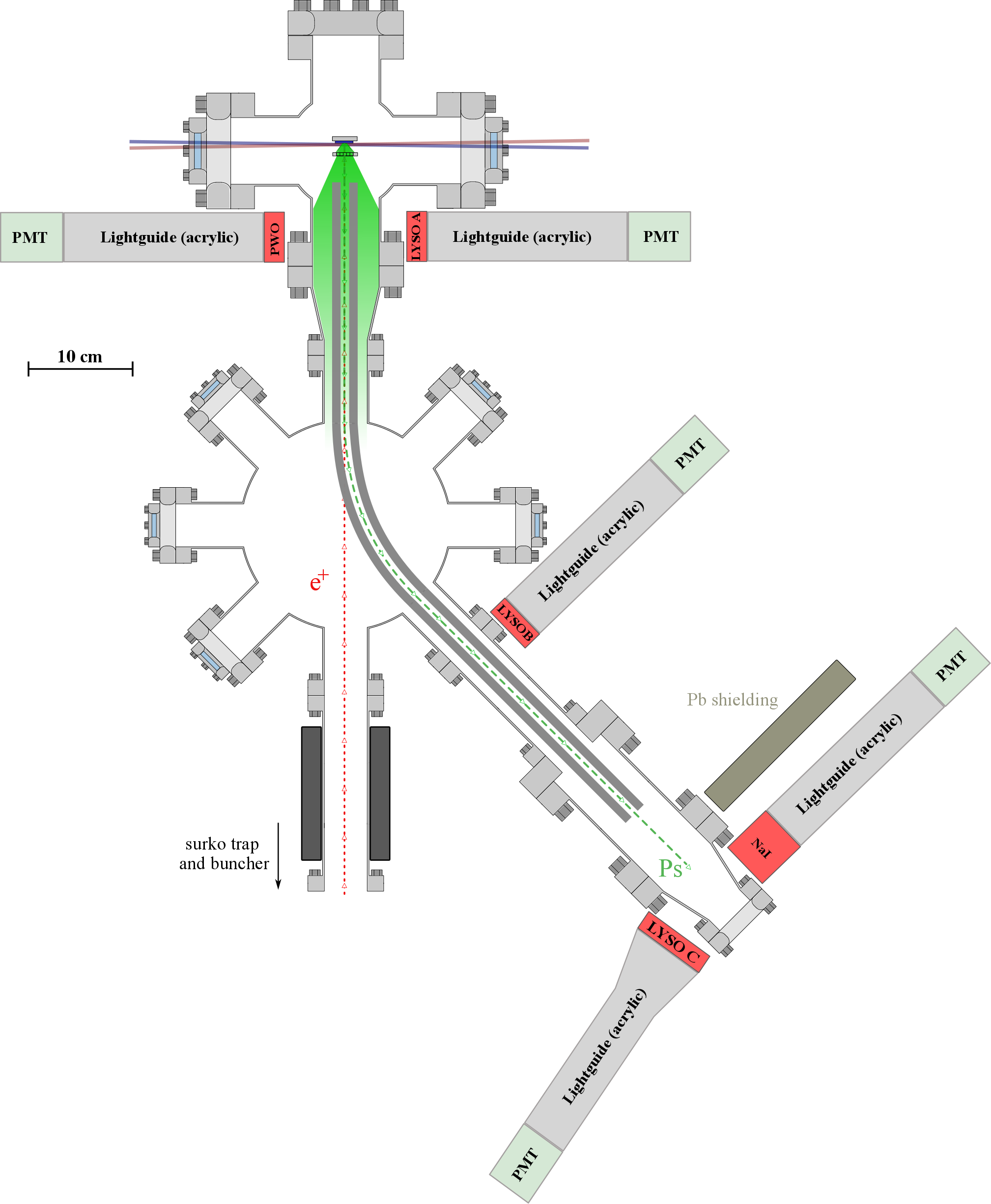
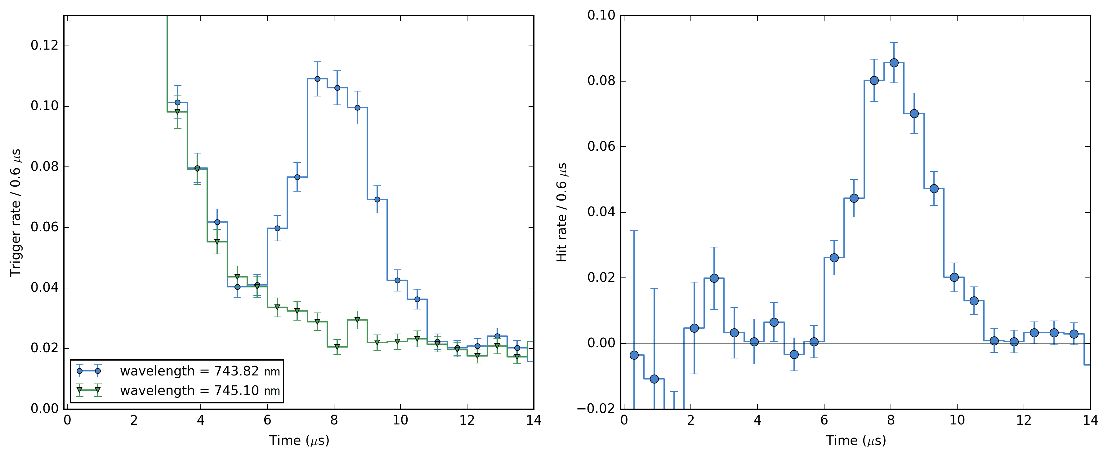
 = 0. If the Ps atoms are then allowed to travel (adiabatically) to a region of zero nominal electric field (our experimental set-up [
 (1)
(1) , which represents not a particle but a wavefunction. That is, the SWE describes how this wavefunction (whatever it may be) will behave. This is not the same thing at all as describing, for example, the trajectory of a particle. Exactly what a wavefunction is remains to this day rather mysterious. For many years it was thought that the wavefunction was simply a handy mathematical tool that could be used to describe atoms and molecules even in the absence of a fully complete theory (e.g., Bohm 1952). This idea, originally suggested by de Broglie in his “pilot wave” description, has been disproved by numerous ingenious experiments (e.g., Aspect et al., 1982). It now seems unavoidable to conclude that wavefunctions represent actual descriptions of reality, and that the “weirdness” of the quantum world is in fact an intrinsic part of that reality, with the concept of “particle” being only an approximation to that reality, only appropriate to a coarse-grained view of the world. Nevertheless, by following the rules that have been developed regarding the application of the SWE, and quantum physics in general, it is possible to describe experimental observations with great accuracy. This is the primary reason why many physicists have, for over 80 years, eschewed the philosophical difficulties associated with wavefunctions and the like, and embraced the sheer predictive power of the theory.
 (2)
(2) and energy by
  and so on. The first term of eq (1) represents the total energy of the system, and is also known as the Hamiltonian, H. Thus, the SWE may be written as
 (3)
(3) (4)
(4) (5)
(5) we find we have to deal with the square root of an operator, which, as it turns out, requires some mathematical sophistication. Moreover, in quantum physics we must deal with operators that act upon complex wavefunctions, so that negative square roots may in fact correspond to a physically meaningful aspect of the system, and cannot simply be discarded as might be the case in a classical system.
 (6)
(6) (7)
(7) have to be four-component matrices to satisfy the equation. That is, the Dirac equation is really a matrix equation, and the wavefunction it describes must be a four component wavefunction. Although there are no problems with negative probabilities, the negative energy solutions seen in the KGE remain. These initially seemed to be a fatal flaw in Dirac’s work, but were overlooked because in every other aspect the equation was spectacularly successful. It reproduced the hydrogen atomic spectra perfectly (at least, as perfectly as it was known at the time) and even included small relativistic effects, as a proper relativistic wave equation should. For example, when the electromagnetic interaction is included the Dirac equation predicts an electron magnetic moment:
 (8)
(8) is known as the Bohr magneton. This expression is also in agreement with experiment, almost: it was later discovered that the magnetic moment of the electron differs from the value predicted by eq (8) by about 0.1% (Kusch and Foley 1948). The fact that Dirac’s theory was able to predict these quantities was considered to be a triumph, despite the troublesome negative energy solutions.
 (9)
(9)
 (10)
(10) represents the negative energy solutions that have caused so much trouble. The existence of these states is central to the theory they cannot simply be labelled as “unphysical” and discarded. The complete set of solutions is required in quantum mechanics, in which everything is somewhat “unphysical”. More properly, since the wavefunction is essentially a complex probability density function that yields a real result when its absolute value is squared, the negative energy solutions are no less physical than the positive energy solutions; it is in fact simply a matter of convention as to which states are positive and which are negative. However you set things up, you will always have some “wrong” energy states that you can’t get rid of. Thus, Dirac was able to eliminate the negative probabilities and produce a wave equation that was consistent with special relativity, but the negative energy states turned out to be a fundamental part of the theory and could not be eliminated, despite many attempts to get rid of them.
