From antihydrogen to positronium spectroscopy

Introduction and PhD motivation

As a new member of the group I would like to introduce myself and my background in physics: I am Andi, coming from Vienna, where I did my bachelors and masters degree in physics at the University of Vienna. Since 2019 I’ve been doing my PhD at the Stefan Meyer Institute for subatomic physics in Vienna as part of the ASACUSA-Cusp (Atomic Spectroscopy And Collision Using Slow Antiprotons) collaboration in the antiproton decelerator (AD) facility at CERN.

The ASACUSA-Cusp experiment aims to measure a property called the hyperfine splitting of antihydrogen [1]. Antihydrogen (\overline{\text{H}} ) is the antiatom of hydrogen, consisting of a positron (e+) and an antiproton (\overline{\text{p}} ), i.e. the antiparticles of electrons and protons, respectively. An antiparticle has the same mass and same absolute charge value as the matter-particle, but opposite sign of the electric charge and magnetic moment. As an example the antiproton has a charge of -1 while the proton has a charge of +1, but both have the same mass. A fundamental property of antimatter is that if it comes close to its matter counterpart both will annihilate and produce a photon. According to the current model of particle physics, the Standard Model, matter-antimatter pairs can be produced by high-energy interactions (the famous formula for the equivalence of energy and mass E = m c2 makes that possible). The energy available for the production of a particle-antiparticle pair must be at least the energy equivalent to the mass of the particles produced, for example to produce an electron-positron pair you need at least 2\times511 = 1022 keV of energy. However, they would annihilate again if not separated. This creation-annihilation processes occurred at short times after the Big Bang but must have stopped at some point as we are living in a universe built from matter. Which leads to the question: Where did the antimatter go?

As hydrogen is the most investigated element it opens the possibility to compare properties to antihydrogen to look for differences, which could give a hint for physics beyond the standard model (in the case of the ASACUSA experiment the framework used is called Standard Model Extension [2,3], but that goes deeply into quantum field theory and will not be further described), which might explain the missing antimatter in our universe.

Experimental setup

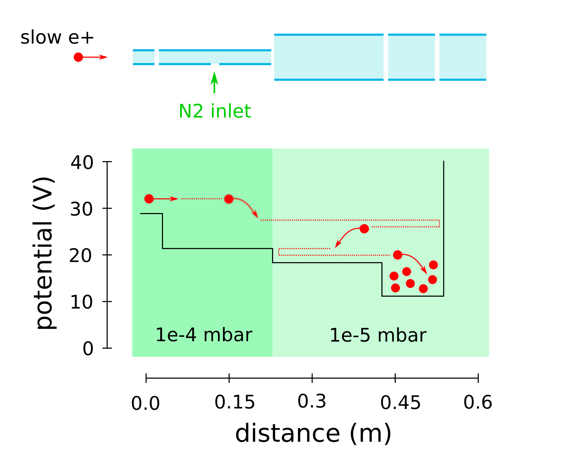
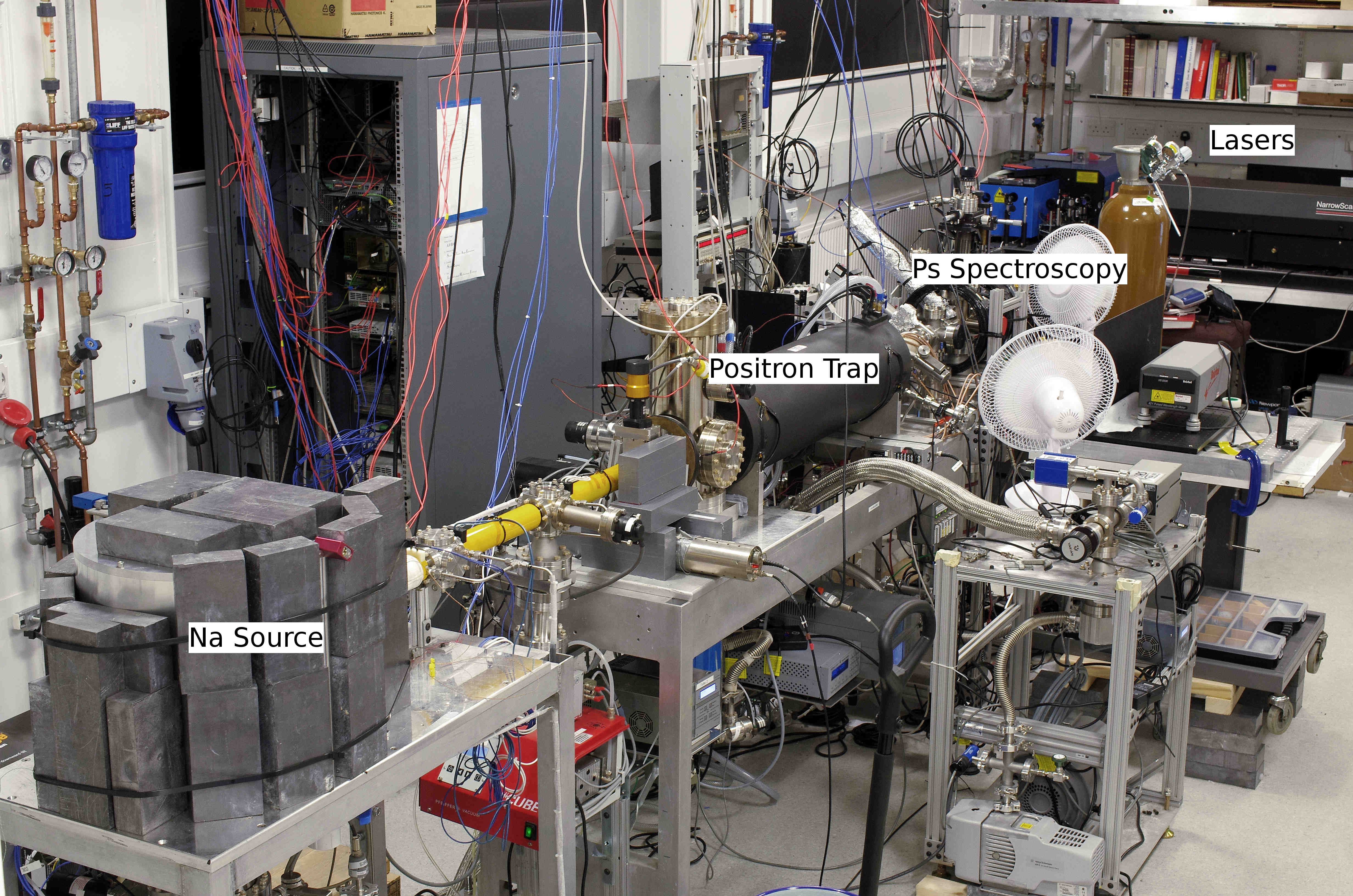
The experimental setup is sketched in Fig.1. (I will not go into detail about the spectroscopy setup as it was not used during my time in the collaboration, but for further information you can look up “Rabi experiment” or have a look at the original publication [4]). The positrons come from a 22Na source, are moderated by a solid Ne moderator[5], and are accumulated in a so-called Buffer Gas Trap [6]. This is done the same way as the Positronium experiments here at UCL, for more information click here. Antiprotons are produced at CERN via the process \text{p} + \text{p} \rightarrow \text{p} + \text{p} + \text{p} + \overline{\text{p}} by shooting high energy protons at tungsten and iridium targets. The energy of the incoming proton must be higher than two times the rest mass of the proton to produce the additional proton-antiproton pair. As the particles have different charge, they can be separated easily by an electric field, protons going one way and antiprotons going the other. The antiprotons can be decelerated afterwards in two rings (the AD and ELENA) to about 100 keV.

Fig.1: Sketch of the ASACUSA experiment. The positrons (red) and antiprotons (blue) are used to produce antihydrogen (purple). Shown are the positron system, the antiproton trap (MUSASHI), the antihydrogen production trap (double-CUSP), the spin-flip cavity, the analysing sextupole and the detector. From Reference [7].

The main process to form antihydrogen is called three-body recombination (\text{e}^+ + \text{e}^+ + \overline{\text{p}} \rightarrow \overline{\text{H}} + e^+ ). That means that a large number of positrons (a few million) and antiprotons (a few hundred of thousand) have to be close together. That is achieved in so-called Penning-Malmberg traps, which is a slightly modified version of a real Penning trap (but the same methods are used). A Penning-Malmberg trap consists of a stack of typically cylindrical electrodes on which different voltages can be applied, producing an on-axis potential (as indicated in Fig.2). Particles with energies lower than the potential barrier cannot escape axially. However, they are pushed towards the wall of the electrodes radially. To counteract this movement, a magnetic field parallel to the electrodes is applied (depending on the purpose of the trap the magnetic field can vary from a few mT up to several T). The particles have no option to escape from the trap, neither axially nor radially, hence they are trapped in a specific region.

Sketch of a Penning-Malmberg trap. The magnetic and electric field as well as a sketch of the on-axis potential along the trap are shown.

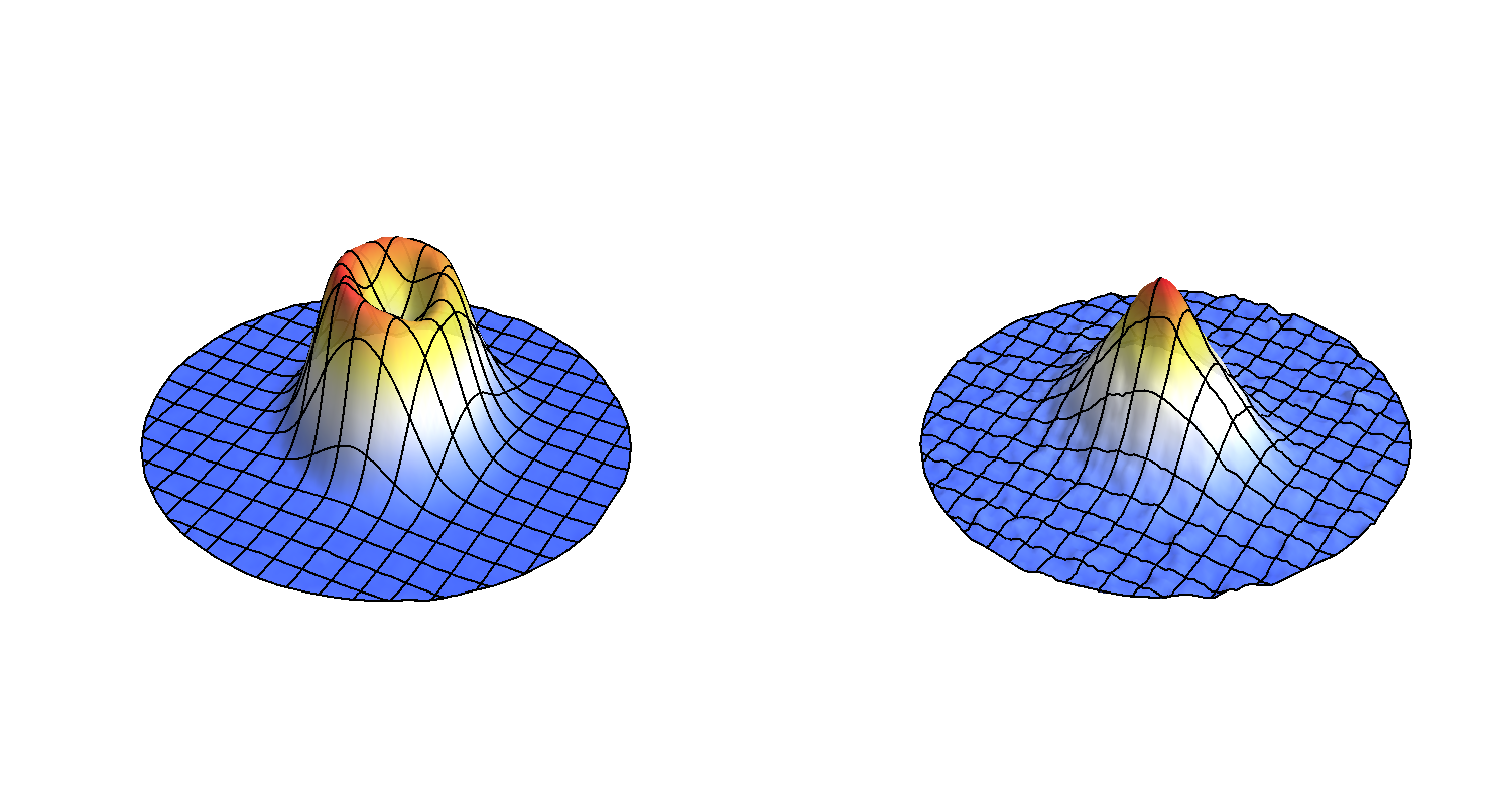
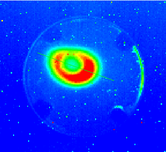
By using this type of trap it is possible to accumulate high numbers of particles with the same charge (e.g. positrons). When a certain density is reached, the particles start to act as an ensemble, which is called a non-neutral plasma. For the production of antihydrogen typically non-neutral plasmas of positrons are needed. By having positrons and antiprotons in the same trap it possible to get an overlap of the positron and antiproton plasmas and the antihydrogen production reaction can start. As antihydrogen is electrically neutral, it can leave the trap and a measurement can be performed.

My previous work

During my PhD my focus lay in upgrading the positron system. I replaced the previous moderation system and buffer gas trap, commissioned an additional trap for accumulating a high number of positrons and optimised the systems. Additionally, I have participated in the design phase, assembly and testing of the new antihydrogen production trap. A further part of my work was the optimisation of the positron plasma before the production of antihydrogen in this trap.

As the AD is not operating all the time, i.e. there are periods when no antiprotons are delivered, the ASACUSA collaboration designed, built and commissioned a low energy proton source [8]. With this source it is possible to use the same apparatus to produce hydrogen when no antiprotons are available for optimising the production scheme. The installation, testing and optimisation of the proton source in the experiment was another part of my PhD.

Future project

As a research fellow I am working in the group of David to set up an experiment to measure the influence of gravity on Rydberg positronium. The first step will be to build a new positron beamline, similar to the one I used at CERN. In parallel we are designing the apparatus for bending positronium upwards using an electric field. This will be a first milestone for the experiment, but that will be expanded upon in a different blog entry.

References

[1] E. Widmann, R. Hayano, M. Hori, and T. Yamazaki, “Measurement of the hyperfine structure of antihydrogen”, Nuclear Instruments and Methods in Physics Research Section B: Beam Interactions with Materials and Atoms, vol. 214, pp. 31–34, 2004. Low Energy Antiproton Physics (LEAP’03).

[2] D. Colladay and V. A. Kostelecký, “Lorentz-violating extension of the standard model,” Phys. Rev. D, vol. 58, p. 116002, Oct 1998.

[3] V. A. Kostelecký and A. J. Vargas, “Lorentz and cpt tests with hydrogen, antihydrogen, and related systems,” Phys. Rev. D, vol. 92, p. 056002, Sep 2015.

[4] I. I. Rabi, S. Millman, P. Kusch, and J. R. Zacharias, “The molecular beam resonance method for measuring nuclear magnetic moments. the magnetic moments of 3Li6, 3Li7 and 9F19,” Phys. Rev., vol. 55, pp. 526–535, Mar 1939.

[5] J. Mills, A. P. and E. M. Gullikson, “Solid neon moderator for producing slow positrons,” Applied Physics Letters, vol. 49, pp. 1121–1123, 10 1986.

[6] T. J. Murphy and C. M. Surko, “Positron trapping in an electrostatic well by inelastic collisions with nitrogen molecules,” Phys. Rev. A, vol. 46, pp. 5696–5705, Nov 1992.

[7] B. Kolbinger, et al., “Measurement of the principal quantum number distribution in a beam of antihydrogen atoms,” The European Physical Journal D, vol. 75, p. 91, Mar 2021.

[8] A. Weiser, A. Lanz, E. D. Hunter, M. C. Simon, E. Widmann, and D. J.Murtagh, “A compact low energy proton source,” Review of Scientific Instruments, vol. 94, p. 103301, 10 2023.

UCL positronium spectroscopy beamline (the first two years)

The UCL Ps spectroscopy positron beamline began producing low-energy positrons almost two years ago, and it has since become slightly longer and somewhat more sophisticated. Though it’s not the most complex scientific machine in the world (compared to, e.g., the LHC) we still find regular use for a 3D depiction of it.  Our model is essentially a cartoon. Typically we use it to create (fairly) accurate schematics that help us to convey the configuration of our equipment at conferences or in publications.

UCL_positron_trap

The snap shot above shows the three main components of the beamline, namely the positron source (left), Surko trap (centre, cross-section), and Ps laser-spectroscopy region (right).  The 3D model is built from simplified forms of the various vacuum chambers and pumps, magnetic coils, and detectors.  And it shows where these all are in relation to one another.  The 45° angled line is being used right now for Rydberg Ps time-of-flight measurements.  The source and trap are based on the design developed by Rod Greaves and Jeremey Moxom of First Point Scientific Inc. (unfortunately now defunct).  You can read about the details of their design in this article.

To allow you to take a closer look we have created a 3D pdf file that you can download here * (licensed under a Creative Commons Attribution 4.0 License). Be aware we use this for illustration/ communication purposes and it is not an accurate technical model. Nonetheless, using this you can pan, zoom, and rotate around our virtual lab to your heart’s content! No need for 3D glasses, though you will need a recent copy of Adobe reader,  (the interactive features probably won’t work in your web browser).

*MD5 checksum c6028573596c9511d9ba0450cd2caa05

And here’s how the lab looks in real life,

beamline_2016_3


Positrons are cool (thanks to tetrafluoromethane)

The positronium spectroscopy experiments we perform are contingent on our ability to form and bunch dense clouds of positrons (anti-electrons).  These are implanted into porous silica where they pair up with electrons and form our favourite exotic element, Ps (which we then photo-ionise with lasers before the two components have chance to annihilate one another).

It’s been 24 years since the first buffer-gas trap [1] was used to collect positrons using a combination of electric and magnetic fields in a configuration known generically as a Penning trap.  The positron accumulation device is often termed a ‘Surko Trap’ after its inventor Cliff Surko, and there’s detailed information about how they work on his site.

The magnetic field lines of a solenoid guide a low-energy positron beam through a series of cylindrical electrodes that have been biased with voltages to create an electric potential minimum (along the axis of the magnetic field) –  see figure below.  These fields alone are not enough to capture positrons from the beam, as those particles with enough energy to enter the trap can also escape it.  Admitting a small amount of nitrogen into the vacuum chamber allows positrons to lose energy as they traverse the trap via inelastic collisions with the buffer-gas molecules, resulting in confinement.  Unfortunately positrons are also lost to annihilation with electrons in the gas.  Surko traps feature several sections with the pressure in each optimised to either capture (higher pressure: good chance of an inelastic collision) or to keep (lower pressure: less chance of annihilation) positrons, which gives the trap its characteristic asymmetric shape.  Thanks to years of optimisation and refinements [2] these devices can accumulate hundreds of millions of positrons from a small radioactive source in just a few minuets (our fairly small trap is capable of capturing roughly half a million e+ in 1 s).  Pulsing the electrode voltages ejects the positrons from the trap in a dense, time-focussed (<10 ns) cloud that’s ideal for creating Ps atoms.

The details of how the positrons interact with the nitrogen are critical for optimisation of the trap.  The likelihood that a positron will have a collision with a nitrogen molecule is related to the pressure of the gas and the scattering cross-section: a hypothetical area that describes the apparent “size” of the molecule.   The scattering cross-section has numerous components that correspond to different types of interaction (elastic collisions, various types of inelastic collisions, ionisation, direct annihilation, Ps formation, …. etc) with some interactions more likely than others.  However, these cross-sections can vary significantly depending on the energy of the collision.

Nitrogen is used in Surko traps because there is a small range of energies  (around 10 eV) where inelastic scattering by exciting an electronic transition in the molecule is reasonably probable, compared to annihilation.  After the positrons cool below the energy needed to excite the electronic transition, further cooling relies on exciting the vibrational states of the molecule, for which the cross-section is rather small.  To speed up cooling we use a second gas, tetrafluoromethane (CF4), which has a much larger cross-section for low-energy inelastic collisions with positrons [3].

Recent Monte Carlo simulations of Surko traps offer a way to further optimise and improve trap designs without the need to manufacture dozens of prototypes.

benc_15

This past week Srdjan Marjanovic, a PhD student at the University of Belgrade, visited UCL to test some of the simulations he has been working on  (see above) using our positron trap.  One suggestion he made is to use CF4 for trapping, in lieu of nitrogen, the logic being that for the energies where inelastic collisions dominate many loss mechanisms are suppressed.  The main difficulty, however, is that many more collisions are needed to successfully capture the positrons, as the energy exchanged to excite vibrational transitions in CF4 is roughly 40 times less than for the electronic transition usually exploited with N2.  Unfortunately  we were unable to adapt our trap to work efficiently with CF4. Nonetheless, by trying we have learnt more about how our trap works and – most importantly –  Srdjan has new data he can use to refine his simulations.

Photo.  Srdjan hard at work on the positron beam.

IMG_20150223_172039

Refs.
[1] Surko, C.M., Wysocki, F.J., Leventhal, M. and Passner, A. (1988). Accumulation and storage of low energy positrons. Hyperfine Interactions, 44:185–200. http://dx.doi.org/10.1007/BF02398669

[2] Surko, C.M. and Greaves, R.G. (2004). Emerging science and technology of antimatter plasmas and trap-based beams. Physics of Plasmas, 11(5):2333. http://dx.doi.org/10.1063/1.1651487

[3] Natisin, M.R., Danielson, J.R. and Surko, C. M. (2014) Positron cooling by vibrational and rotational excitation of molecular gases. J. Phys. B 47: 225209. http://dx.doi.org/10.1088/0953-4075/47/22/225209

Positron beams, then and now

There have been positron beams in use at UCL since the early 1970’s since the first efficient positron moderator was discovered there by Paul Coleman, Karl Canter and co-workers [http://iopscience.iop.org/0022-3700/5/8/007]. The photograph below was taken in 1996, and shows a positron beam used in Dr David Cassidy’s PhD thesis (Positronium formation at surfaces and studies towards the production of cold antihydrogen, supervisor Mike Charlton, 1999). This beam, which is no longer operational, used a tungsten mesh grid as a moderator and produced around 1000 positrons/second. One can see a large diffusion pump at the lower end, and the black magnet coils used to guide the beam.
2215_001
Things have changed quite a lot since those days. The current setup in our lab (shown below) at the moment uses a rare gas solid moderator (neon) and produces more than 5 million positrons/second. There are four main sections to this beamline, (1) the shielded Na source and moderator that produces positrons, (2) the positron buffer gas trap that provides the pulsed beam (5 ns wide pulses with 500,000 positrons each), (3) the Ps spectroscopy chamber where our Ps producing silica target is placed and (4) the laser table, where our Nd:YAG pumps our Sirah pulsed dye laser and our Radiant pulsed dye laser. Together all these components are used to produce Rydberg positronium in a two step photon process. There are no more diffusion pumps to be found!

lab_2

Trapped positrons

We have trapped positrons, and slowed and cooled them by collisions with N_2 buffer gas and CF_4 cooling gas. The images are 3D plots of the positrons detected on a phosphor screen (see banner at the top of the page).

densityPlots

The left-hand image shows the image resulting from the positron beams impinging on the phosphor screen, passing directly through the trap. The trap shows the distribution with a dip in the centre (see this post for an explanation of where this comes from). The right-hand image was generated by accumulating and cooling positrons in the trap for 1 second. The cloud of trapped positrons is then bunched and accelerated out of the trap and onto the screen.

Next step: we will accelerate these positrons onto a porous target and make positronium!

Positron beam

We have built a dc beam of positrons. After moderation in solid neon the positrons are magnetically guided away from the source,  through what will be our buffer gas trap, and onto a phosphor screen, located in front of a CCD camera.

Below is a typical image we have recorded of our positron beam.

positrons12May14

The beam has a roughly doughnut-shape, which is determined by the shape of the neon moderator (the moderator has a hollow centre, and so there are fewer of the slow positrons that we detect in the centre of the beam). This beam structure is highlighted in the following figure which shows the recorded beam intensity along a line (shown in the above figure).

positrons12May14

In this experiment we are recording around 2 million positrons per second, several metres downstream of the source.

This is an important step forward in our experiment. The next step will be to accumulate positrons in our trap, and then accelerate them onto a target for Ps production.