Controlling Positronium Annihilation with Electric Fields

To produce Rydberg (highly-excited) states of positronium we use a multi-photon $1 ^3S \rightarrow 2 ^3P \rightarrow nS/nD$ excitation scheme [1]. These high- $n$ Ps atoms are long-lived and could potentially be used for (anti)-gravity measurements, however, the intermediate state ( $n=2$ ) has interesting properties of it’s own, as described in our latest article (Phys. Rev. Lett. 115, 183401 ).

Unlike regular atoms, Ps has the peculiar feature that it can self-annihilate into gamma-rays. The amount of overlap between the positron and electron wave functions depends on the particular state the atom is in, and this determines how long before self-annihilation occurs (characterised by the average annihilation lifetime). The quantum spin ( $s=1/2$ ) of the electron and positron can combine in positronium to either cancel ( $S=0$ ) or sum ( $S=1$ ), depending on the relative alignment between the two components. In the former case (para-Ps) the atom has a very short ground-state lifetime of just 125 ps, whereas in the latter case (ortho-Ps) the atom lives in the $n=1$ state for an average of 142 ns (this may not sound very long but it’s actually plenty of time to do spectroscopy with pulsed lasers).

We produce $n=1$ ortho-Ps ( $1^3S_1$ ) atoms then excite these using 243 nm laser light from our UV laser. The electronic dipole transition selection rules (principally, $\Delta S= 0$ and $\Delta \ell = \pm 1$ ) dictate that this single-photon transition drives the atoms to the $n = 2$ , $\ell= 1$ , $S= 1$ state ( $2 ^3P_J$ ). For historical reasons the orbital angular momentum is written here as $S$ ( $\ell= 0$ ) and $P$ ( $\ell= 1$ ).

The fluorescence lifetime of an excited atom is the time it takes, on average, to spontaneously emit a photon and decay to a lower energy state. All of the $n=2, \ell = 1$ states have a fluorescence lifetime of 3.19 ns, and an annihilation lifetime of over 100 $\mu$ s (practically infinite compared to the time-scale of our measurements, i.e., $2^3P$ states don’t annihilate directly, but can decay to a different state then annihilate). The $n=2, \ell = 0$ ortho and para states have annihilation lifetimes of 1136 ns and 1 ns, and they both fluoresce with a lifetime of $\simeq$ 0.24 s ( $\approx \infty$ ). The bottom line here is that there are a wide range of fluorescence and annihilation lifetimes for the various possible sub-states in the $n=1$ and $n=2$ manifolds.

In a magnetic field the short-lived $S=0$ and longer-lived $S=1$ states (with the same $\ell$ ) are mixed together (Zeeeman mixing). Similarly, an electric field mixes states with different $\ell$ (but the same $S$ ) (Stark mixing). By exciting Ps to $n = 2$ in a weak magnetic field then varying an electric field, we can tailor the extent of this mixing to increase or decrease the overall lifetime. This technique can be used to greatly increase the excitation efficiency to another state, since the losses due to annihilation can be reduced. Conversely, increasing the annihilation rate can be used as an efficient way to detect excitation.

The polarization orientation of the UV excitation laser gives us some control over which $M_J$ states are subsequently populated. More specifically, if the laser polarization is parallel to the applied magnetic field then only $\Delta M_J=0$ transitions are allowed, whereas if the polarization is perpendicular to it then $\Delta M_J$ must change by $\pm 1$ .

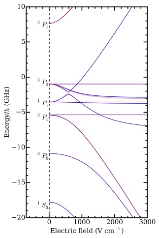
Below is a calculation of how the $n=2$ energy levels are shifted by an electric field, in zero magnetic field (red) and in a magnetic field of 13 mT (blue). Note the avoided crossing at 585 V/ cm in the 13 mT case.
StarkmapFig So what can we actually measure? In most cases, laser excitation makes it more likely for ground state ortho-Ps to ultimately end up in the short-lived para-Ps state, thus applying the laser causes an increase in the annihilation gamma ray flux at early times. This change can be observed and quantified using the parameter $S$ (higher values means more gamma rays were detected compared to a measurement made without the laser). This is plotted below for various electric field strengths, and with the laser polarised either parallel (red) or perpendicular (green) to the magnetic field. In both cases, the avoided crossing gives a sharp increase in annihilation rate (see the “ears” in both plots), whilst higher electric fields either reduce or increase the signal, depending on which $M_J$ states the laser initially populates.

Quenching

Notice that when the laser polarisation is aligned parallel to the magnetic field (red), very high electric fields lead to negative $S$ values. This means that the lifetime of the Ps becomes longer than 142 ns (the ground-state ortho-Ps lifetime) if the laser is applied. This is due to the fact that in this field configuration there is significant mixing into the long lived $2^3S_1$ state. This could be used to produce an ensemble of pure $2^3S_1$ states, by exciting Ps in this high field and then extracting the excited state into a region of zero field. These pure states could be exploited for $n=2$ microwave spectroscopy [3].